Gobierno de
la ciudad de Buenos Aires
Hospital Neuropsiquiátrico
"Dr. José Tiburcio Borda"
Laboratorio
de Investigaciones Electroneurobiológicas
y
Revista
Electroneurobiología
ISSN: 0328-0446
![]()
The Nervous Principle:
Active versus
Passive Electric Processes In Neurons
by
Danko Dimchev Georgiev, M.D.
Division
of Electron Microscopy, Medical University of Varna, Varna 9000, BULGARIA
Correspondencia / Contact: dankomed@SoftHome.net
Electroneurobiología 2004; 12 (2), pp. 169-230; URL: http://electroneubio.secyt.gov.ar/index2.htm
Copyright
© 2004 del autor / by the author. Esta es una investigación
de acceso público; su copia exacta y redistribución por cualquier medio están
permitidas bajo la condición de conservar esta noticia y la referencia completa
a su publicación incluyendo la URL original (ver arriba). / This is an Open
Access article: verbatim copying and redistribution of this article are
permitted in all media for any purpose, provided this notice is preserved along
with the article's full citation and original URL (above).
Acceso de red permanente: puede obtener un archivo .PDF (2 Mb: recomendado) o .DOC (1,5 Mb)
para imprimir esta investigación, de / You can download a .PDF
(2 Mb, recommended) or a .DOC file (1.5 Mb) for printing, from http://electroneubio.secyt.gov.ar/index2.htm
También como archivo .htm comprimido / Also as a compressed-htm .ZIP file
Abstract
This essay presents in
the first section a comprehensive introduction to classical electrodynamics. The
reader is acquainted with some basic concepts like right-handed coordinate
system, vector calculus, particle and field fluxes, and learns how to calculate
electric and magnetic field strengths in different neuronal compartments.
Then the exposition comes to explain the basic difference
between a passive and an active neural electric process; a brief historical
perspective on the nervous principle is also provided. A thorough description is
supplied of the nonlinear mechanism generating action potentials in different
compartments, with focus on dendritic electroneurobiology. Concurrently, the
electric field intensity and magnetic flux density are estimated for each
neuronal compartment.
Observations are then discussed, succinctly as the
calculated results and experimental data square. Local neuronal magnetic flux
density is less than 1/300 of the Earth’s magnetic
field, explaining why any neuronal magnetic signal would be suffocated by the
surrounding noise. In contrast the electric field carries biologically important
information and thus, as it is well known, acts upon voltage-gated transmembrane
ion channels that generate neuronal action potentials. Though the transmembrane
difference in electric field intensity climbs to ten million volts per meter,
the intensity of the electric field is estimated to be only ten volts per meter
inside the neuronal cytoplasm.
Principio del funcionamiento nervioso: oposición de procesos eléctricos activos y pasivos en las neuronas
Sumario
Este trabajo presenta en su primera
sección una introducción general a la electrodinámica clásica. Cubre los
temas electroneurobiológicos introductorios de la mayoría de los cursos de
neurociencias, asegurando ante todo la familiaridad del estudiante con los
sistemas de coordenadas a mano derecha, así como con el cálculo de vectores y
con los flujos de partículas y de campo. En esta sección el lector aprende a
calcular las intensidades de campo eléctricas y magnéticas dentro de los
diferentes compartimientos neuronales.
Luego la exposición se aboca a
explicar la esencial diferencia entre procesos neuroeléctricos pasivos y
activos; se provee también una breve perspectiva histórica sobre el principio
o fundamento de la función neural. Proporciónase una descripción detallada de
los mecanismos no lineares que generan potenciales de acción en los diferentes
compartimientos, con énfasis en la electroneurobiología dendrítica.
Concurrentemente se estiman la intensidad de campo eléctrico y la densidad de
flujo magnético para cada compartimiento neuronal.
Las observaciones son entonces analizadas, sucintamente por cuanto los resultados calculados cuadran bien con los datos experimentales. La densidad local del flujo magnético es menos que 1/300 de la del campo magnético terrestre, lo que explica por qué cualquier señal magnética útil es sofocada por el ruido ambiental. En contraste, el campo eléctrico porta información biológicamente relevante y, como es muy bien sabido, actúa sobre canales iónicos transmembranales abiertos y cerrados por voltaje, que controlan el potencial de acción de la célula. Aunque la diferencia en la intensidad del campo eléctrico a través de la membrana asciende a diez millones de voltios por metro y aun más, la intensidad del campo eléctrico se estima en sólo diez voltios por metro dentro del citoplasma neuronal.
Нейронный принцип: сравнительное описание активных и пассивных электрическиx процесcов
Резюме
Первая
часть
представляет
собой
краткое
введение в
класическую
электродинамику.
Здесь
приведены
общие
положения,
излагаемые
во многих
учебниках
физики:
правоориентированная
координатная
система,
векторноe
исчисление,
поток из
частиц и
полевый
поток. В этой
части
читатель
знакомится
со способами
вычисления
интенсивности
электрического
и магнитного
поля в
различных
структурах
нервной
клетки.
Во
второй части
объясняется
различие
между
активными и
пассивными
электрическими
процессами в
нейронах. Эта
проблема
рассматривается
также в
историческом
аспекте.
Представлено
подробное
описание
нелинейных
механизмов
генерации
действующих
потенциалов
в отдельных
структура
нервной
клетки, и
особенно
электронейробиологии
дендритов.
Для каждого
органа
клетки (дендриты,
сома, аксон)
вычислены
интенсивности
электрического
и магнитного
поля.
Полученные результаты соответствуют экспериментальным данным. Плотность локального магнитого потока нейронов составляет менее 1/300 плотности магнитного потока Земли. Поэтому шум среды подавляет магнитный сигнал нейрона. Напротив, электрическое поле несет биологически значимую информацию и оказывает влияние на зависящие от разности потенциалов ионные каналы которые генерируют действующие потенциалы нейронов. Несмотря на то, что трансмембранное электрическое поле достигает 10 миллионов В/м, в нейронной протоплазме интенсивность электрического поля составляет лишь 10 В/м.
Table of Contents
1.1 Right-handed coordinate systems
2 Electric and magnetic fields in neurons
2.1 Passive electric properties – cable equation
2.1.1 Spread of voltage in space and time
2.1.2 Assessment of the electric field intensity
2.1.3 Propagation of local electric currents
2.2 Active electric properties – the action potential
2.2.1 Nernst equation and diffusion potentials
2.2.2 Resting membrane potential
2.2.3 Generation of the action potential
2.3.1 Electric intensity in dendritic cytoplasm
2.3.2 Electric currents in dendrites
2.3.3 Magnetic flux density in dendritic cytoplasm
2.3.4 Active dendritic properties
2.5.1 The Hodgkin-Huxley model of axonal firing
2.5.2 Passive axonal properties
2.5.3 Electric intensity in the axonal cytoplasm
2.5.4 Magnetic flux density in axonal cytoplasm
2.6 Electric fields in membranes
In order to investigate the electromagnetic field structure
in neurons it behooves to be acquainted with the basic mathematical definitions
and physical postulates in classical electrodynamics. Before anything else, it
is worth pointing out that a quantity is either a vector or a scalar. Scalars
are quantities fully described by a magnitude alone. Vectors are quantities
fully described by both a magnitude and a direction. Because we will work mostly
with vectors we have to define what is positive normal to a given surface s,
what is the positive direction of a given contour Γ and what is a
right-handed coordinate system.
Right-handed coordinate system Oxyz is such a system in
which if the z-axis points toward your face the counterclockwise rotation of the
Ox axis to the Oy axis has the shortest possible path. The positive normal +n of
given surface s closed by contour Γ is collinear with the Oz axis of
right-handed coordinate system Oxyz whose x- and y-axis lie in the plane of the
surface. The positive direction of the contour Γ is the direction in which
the rotation of x-axis to the y-axis has the shortest possible path (Zlatev,
1972).

FIG 1 Left: Direction of the positive normal +n and the positive
direction of the contour Γ. Right: Right handed coordinate system Oxyz.
After that, for working with vectors it should be noted
that there are two types of multiplication of vectors - the dot product and the
cross product. Geometrically, the dot product of two vectors is the magnitude of
one times the projection of the other along the first. The symbol used to
represent this operation is a small dot at middle height (·), which is where
the name dot product comes from. Since this product has magnitude only, it is
also known as the scalar product:
where b
is the angle between the two vectors.
Geometrically, the cross product of two vectors is the area
of the parallelogram between them. The symbol used to represent this operation
is a large diagonal cross (×), which is where the name cross product comes
from. Since this product has magnitude and direction, it is also known as the
vector product:
where the vector  is a unit vector perpendicular to
the plane formed by the two vectors. The direction of
is determined by the right hand
rule.
is a unit vector perpendicular to
the plane formed by the two vectors. The direction of
is determined by the right hand
rule.
The right hand rule says that if you hold your right hand
out flat with your fingers pointing in the direction of the first vector and
orient your palm so that you can fold your fingers in the direction of the
second vector, then your thumb will point in the direction of the cross product.
The gradient  is a vector operator called Del or
Nabla (Morse & Feshbach, 1953; Arfken,
1985; Kaplan, 1991; Schey,
1997). It is denoted as:
is a vector operator called Del or
Nabla (Morse & Feshbach, 1953; Arfken,
1985; Kaplan, 1991; Schey,
1997). It is denoted as:
f = grad(f)
The
gradient vector is pointing toward the higher values of f, with magnitude equal
to the rate of change of values. The direction of f is the orientation in which the directional derivative has the largest value
and |f| is the value of that directional derivative. The directional derivative
uf(x0,y0,z0) is the rate at which
the function f(x,y,z) changes at a point (x0,y0,z0)
in the direction u.
and  is the unit vector (Weisstein,
2003).
is the unit vector (Weisstein,
2003).
The particle flux is a scalar physical quantity
defined by the expression:
 ,
,
where

dV denotes a volume segment with
length dl that is filled with fluid that for
time
dt passes with velocity v trough any
cross section s of
dV; β is the is the angle between the vectors  and
and  . It is worth to remind that
has the direction of the positive
normal +n, and its magnitude is proportional to the surface area s. Simple
substitution of the expression for
dV
into the expression for
. It is worth to remind that
has the direction of the positive
normal +n, and its magnitude is proportional to the surface area s. Simple
substitution of the expression for
dV
into the expression for  gives us
Thus
we have obtained that the particle flux is a scalar product of two vectors - the
particle velocity vector
 and the surface vector
. In electrodynamics, ion currents in electrolytes and the currents composed of
electrons are the particle fluxes of top neurobiological interest, but
quasiparticles such as solitons and phonons are also modeled.
and the surface vector
. In electrodynamics, ion currents in electrolytes and the currents composed of
electrons are the particle fluxes of top neurobiological interest, but
quasiparticles such as solitons and phonons are also modeled.
We
could define an analogous scalar quantity when we investigate physical fields,
e.g. the field of electromagnetic force or electromagnetic field. There we can
define the field flux as a scalar product of the field intensity  through surface .
The
electromagnetic force field is composed from the forces of electric and magnetic
fields, whose different causal actions can be nonetheless described as mediated
by a single sort of microphysical change-causing energy packets, called photons.
Taking the photons’ action collectively – like as floods can be described by
neglecting the swervings of individual water molecules – the electric field
could be described via the vector field of electric intensity
 . Electric intensity is defined as the ratio of the electric force
  acting upon a charged body and the
charge q of the body:
acting upon a charged body and the
charge q of the body:
It should be noted that the electric field is a potential
field – that is, the work WΓ along closed contour Γ with
any length l is zero:
Every point in the electric field has an electric potential
V defined with the specific (for unit charge) work needed to carry a charge from
this point to infinity. The electric potential of point c of a given electric
field has potential V defined by:
where V∞= K = 0. The electric potential
difference between two points 1 and 2 defines voltage V, whose synonyms are
electric potential, electromotive force, potential, potential difference, and
potential drop:
The link between the electric intensity
and the gradient of the voltage V is:

Another vector, not directly measurable, that describes the
electric field is the vector of electric induction
 . For isotropic dielectrics electric induction is defined as:

where ε is the electric permittivity of the
dielectric. The electric permittivity of the vacuum is denoted as ε0 =
8.84×10⁻¹² F/m.
The Maxwell’s law for the electric flux ФD
of the vector of electric induction says that ФD
through any closed surface s is equal to the located in the space region s
charge q that excites the electric field. This could be expressed
mathematically:
If the normal +n of the surface s and the vector
form angle b,
then the flux ФD could be defined as:

FIG 2 The flux ФD of the vector of the
electric induction
through surface s.
From the Maxwell’s law we could easily derive the
Gauss’ theorem:
where ФE is the flux of the vector of the
electric intensity
through the closed surface s.
It is important to note that the full electric flux ФD
could be concentrated only in a small region Δs of the closed surface s, so
in such cases we could approximate:
In other cases, when the electric field is not concentrated
in such a small region but we are interested in knowing the partial electric
flux ΔФD through partial surface Δs for which is
responsible electric charge Δq, it is appropriate to use the formula:
The electric current
i
, that is the flux of physical charges, could be defined by using both scalar
and vector quantities (Zlatev,
1972):
where
 is the density of the electric
current. As a scalar quantity the current density J is defined by the following
formula:
is the density of the electric
current. As a scalar quantity the current density J is defined by the following
formula:
where sn is the cross section of the current
flux ФJ. It is useful to note that usually by means of i it is
denoted the flow of positive charges. In the description, the flow of negative
charges could be easily replaced by a positive current with equal magnitude but
opposite direction. Sometimes, however, we would like to underline the nature of
the charges in the current. To this purpose we will use vectors with indices,
e.g.
 or
or
 , where the direction of the vectors coincides with the direction of motion of
the negative or positive charges.
, where the direction of the vectors coincides with the direction of motion of
the negative or positive charges.
If we have a cable and a current flowing through it,
according to Ohm's law the current i is proportional to the voltage V and
conductance G and inversely proportional to the resistance R:
where ρ is the specific resistance for
the media, γ is the specific conductance, l is the length of the
cable and s is its cross section.
The
magnetic field is the second component of the electromagnetic field and is
described by the vector of magnetic induction
![]() (also known as: magnetic field
strength or magnetic flux density) that is perpendicular to the vector of the
electric intensity
(also known as: magnetic field
strength or magnetic flux density) that is perpendicular to the vector of the
electric intensity
![]() . The magnetic field does only act on moving charges. It manifests itself via
the magnetic force
. The magnetic field does only act on moving charges. It manifests itself via
the magnetic force
![]() acting upon flowing currents inside
the region where the magnetic field is distributed. From Laplace’s law it is
known that the magnetic force
acting upon flowing currents inside
the region where the magnetic field is distributed. From Laplace’s law it is
known that the magnetic force
![]() , which acts upon an electric current-conveying cable immersed in a magnetic
field with magnetic induction
, which acts upon an electric current-conveying cable immersed in a magnetic
field with magnetic induction
![]() , is equal to the vector product:
, is equal to the vector product:
If we have a magnetic dipole, the direction of the vector
of magnetic induction is from the south pole (S) to the north pole (N) inside
the dipole – and from N to S outside it.
The magnetic field could be excited either via changes in
an existing electric field
![]() or by a flowing electric current
i.
In the first case the magnetic induction is defined by the Ampere’s law (in
case J = 0):
or by a flowing electric current
i.
In the first case the magnetic induction is defined by the Ampere’s law (in
case J = 0):
In the second case, if we have a cable with current i, it
will generate a magnetic field with magnetic induction
![]() whose lines of force have the
direction of rotation of a right-handed screw piercing in the direction of the
current i.
whose lines of force have the
direction of rotation of a right-handed screw piercing in the direction of the
current i.

FIG 3 Direction of the lines of magnetic induction around the
path axis with current (a) and along the axis of contour with current (b). The
current i by convention denotes the flux of positive charges.
The
total electromagnetic field manifests itself with a resultant electromagnetic
force
![]() defined by the Coulomb-Lorentz
formula:
defined by the Coulomb-Lorentz
formula:
![]()
where
![]() is the velocity of the charge q.
is the velocity of the charge q.
If we have magnetically isotropic media, then we could
define another vector describing the magnetic field. It is called magnetic
intensity
![]() , tantamount to
, tantamount to

where μ is the magnetic permeability of the media. The
magnetic permeability of the vacuum is denoted with μ0 = 4π×10-7
H/m.
The circulation of the vector of magnetic intensity along
the closed contour Γ1 with length l, which interweaves in its
core the contour Γ2 with current i flowing through Γ2,
is defined by the formula:
![]()
It can be seen that the magnetic field is a non-potential
field, since the lines of field intensity
![]() are closed and do always interweave
the contour with the excitatory current i. The circulation of the vector
are closed and do always interweave
the contour with the excitatory current i. The circulation of the vector
![]() will be zero only along the closed
contours which do not interweave in their cores any current i (Zlatev,
1972).
will be zero only along the closed
contours which do not interweave in their cores any current i (Zlatev,
1972).

FIG 4 The circulation of the vector of magnetic intensity
![]() along the closed contour Γ1
equals the current i flowing through the interweaved contour Γ2.
along the closed contour Γ1
equals the current i flowing through the interweaved contour Γ2.
Analogously to defining the flux ФD of the
vector of the electric induction
![]() we can define the flux ФB
of the vector of the magnetic induction
we can define the flux ФB
of the vector of the magnetic induction
![]() :
:
![]()
It is useful to know that the change in magnetic flux
generates induced voltage V according to the Lenz’s law:
Thus the Lenz’s law shows that there will be induced
voltage (and therefore electric current) if there is a static cable inside
changing magnetic field:
or if the cable is moving inside a static magnetic field:
![]()
The full magnetic flux ФL of the magnetic
field self-induced by a contour with current i is called self-induced flux. The
self-induced flux is a linear function of the current:
![]()
where L is scalar known as self-inductance and depends only
on the magnetic permittivity μ of the media and the geometric parameters
ΠL that determine the size and the shape of the contour:
L
= f (m
, PL)
Self-induced voltage appears on electric wires every time
that there is a change of the current i – and this self-induced voltage
opposes to the change of the current:
![]()
We have up till now presented the basic principles of
electromagnetism. In order to summarize them it is useful to write down the
Maxwell’s equations. Although these equations have been worked out more than a
century ago they present in concise form the whole electrodynamics. We will
consider two cases: (i) in the absence of magnetic or polarizable media and (ii)
with magnetic and/or polarizable media.
In absence of magnetic or polarizable media the equations
can be written in both forms, i.e. in integral or differential form. They will
be listed on the following table.
Table 1
Maxwell’s equations in the absence of magnetic or polarizable media.
|
Laws |
Integral form |
Differential form |
|
Gauss’ law for electricity |
|
|
|
Gauss’ law for magnetism |
|
|
|
Faraday’s law of induction |
|
|
|
Ampere’s law |
|
|
In the cases where a magnetic and/or polarizable medium
steps in, the above equations must be re-written in order to take into account
the processes occurring inside the medium. We will write down the differential
form of the laws.
The Gauss’ law for electricity takes the form:

where P denotes the polarization. For free space we have D
= e0E
and for isotropic linear dielectric D = e×E.
If a material contains polar molecules, when no electric field is applied they
will generally be in random orientations. An applied electric field will
polarize the material, by orienting the dipole moments of polar molecules. This
decreases the effective electric field between the plates and increases the
capacitance of the parallel plate structure.
The Gauss’ law for magnetism remains in the same form:
![]()
as well as the Faraday’s law of induction:
![]()
The Ampere’s law could rather be written in the form:
where
M denotes the magnetization. For free space we have B = m0H
and for isotropic linear magnetic medium B = mH. In matter the orbital motion of electrons creates
tiny atomic current loops, which produce magnetic fields. When an external
magnetic field is applied to a material, these current loops will tend to align
in such a way as to oppose the applied field. This may be viewed as an atomic
version of Lenz’s law: induced magnetic fields tend to oppose the change,
which created them. The materials whose only magnetic response is this effect
are called diamagnetic. Therefore all materials are inherently diamagnetic, but
if the atoms have some net magnetic moment as in paramagnetic materials, or if
there is long-range ordering of atomic magnetic moments as in ferromagnetic
materials, these stronger effects are always dominant (Nave,
2003).
It is of interest to note that the three basic physical
constants in electromagnetism, namely electric permittivity of vacuum, magnetic
permeability of vacuum and velocity of light in vacuum, are linked by the
equation:
![]()
This
equation exposes a crucial fact, which shows that in electrodynamics the minimal
number of physical units is four: length, time, mass and charge.
Taking into account the presented basic laws of classical
electrodynamics, we could now try to model the electromagnetic field structure
and effects taking place in the different compartments of neural cells -
dendrites, soma and axons.
The earliest ideas about the nature of the signals in the
nervous system, going back to the Greeks, involved notions that the brain
secretes fluids or “spirits” that flow through the nerves into the muscles.
A new era, nevertheless, opened in 1791 when Luigi Galvani of Bologna showed
that frog muscles could be stimulated by electricity (Galvani,
1791). His postulate of the existence of “animal electricity” in
nerves and muscles soon led to a focus of attention almost exclusively on the
electrical mechanisms for nerve signaling.
In 1838 Carlo Matteucci detected currents in the nerves of
the electric fish and pointed out “the greatest analogy that we have between
the unknown force in nerves and that of electricity” (Matteucci,
1838). In the 1840s Matteucci observed that when an amputated
frog’s leg was placed in contact with another leg undergoing contractions, it
would contract as well. Using this organic “device”, Matteucci discovered an
ongoing current in frog muscle, which he could detect with particular clarity in
cases of injury (Matteucci,
1840, 1844).
In spite of these first experimental results, the nature of
the neural signals remained disputable. In early 1841, the Berlin physiologist
and anatomist Johannes Müller presented his twenty-three-year-old medical
student Emil Du Bois-Reymond with Matteuci’s results and asked Du Bois-Reymond
to establish, once and for all, whether the nervous principle was electrical in
nature. Müller himself had his doubts. Several facts suggested a fundamental
difference between neural and electrical signals: (i) a ligated (tied or
crushed) nerve could conduct electricity but could not transmit the nervous
principle, (ii) many other types of stimuli besides electricity could excite
nerves, giving rise to the nervous principle, and (iii) other moist animal
tissues, too, could conduct electricity as suitably as the nervous tissue, if
not better. Du Bois-Reymond was to repeat, verify, and extend Matteuci’s
experiments on the electrical properties of frog muscles. After seven years of
hard work he prepared a comprehensive description (in fact a text of about 800
pages) explaining in minute detail the performed experiments. As an appendix, it
offered an extensive series of plates illustrating the most important
experimental setups, instruments, and frog preparations (Du Bois-Reymond, 1848). In 1850s, Reymond’s slightly younger
colleague Hermann von Helmholtz, later a famous physicist, was able to measure
the speed of conduction of the nerve impulse. He showed for the first time that,
though fast, it is not all that fast. In the large nerves of the frog it moves
at about 40 meters per second, which is about 140 kilometers per hour (von
Helmholtz, 1850; 1852; 1854).
This was another landmark finding, as it showed that the mechanism of the nerve
impulse has to involve something more than merely the physical passage of
electricity as through a wire; it has to involve an active biological process.
Therefore the impulse eventually came to be called action potential.
The ability of a nerve to respond to an electrical shock
with an impulse is a property referred to as excitation. It thus has been
frequent to say that the nerve is excitable. Yet in the earliest experiments
there were no instruments for recording the impulse directly; it could be
detected only by means of the fact that, if a nerve was connected to its muscle,
after a brief period for conduction in the nerve the shock was followed by a
twitch of the muscle. The fleeting nature of the twitch indicated that an
impulse must also occur in the muscle, so that the muscle was also recognized as
having the said property of excitability. The electrical nature of the nerve
impulse and its finite speed of conduction were important discoveries for
physiology in general – indeed, for articulating several fields of scientific
endeavor – because they constituted the first direct evidence for the kind of
activity present in the nervous system.
In addition, the fact that the impulse moves at only
moderate speed had tremendous implications for psychology, for it seemed to
break the mind away from the actions that the mind wills. In effect, it provided
empirical evidence understood as supporting the idea of dualism – namely, that
the mind is separate from the body. It was one of the stepping-stones toward the
development of modern psychology and study of behavior, as well as added fuel
for the debate about the nature and relationships of mind and body (Shepherd, 1994).
Between September 1883 and May 1884 Alberto Alberti kept alive and almost daily mapped an exposed human brain as regards sensations and movements stirred through electricity (Alberti, 1884; 1886; Crocco & Contreras, 1986a; Crocco, 1994; Petrolli, 2001) and since then and until 1912 Richard Sudnik, the researcher that had found the proper values of current used by Alberti (Crocco & Contreras, 1986b), published some fifty research papers on electrotherapeutics including probings in the electrical nature of the nervous principle. His friend d'Arsonval (1896) observed phosphenes, dizziness and some people fainting away as their head got into an induction coil and in 1902, in Wien, Bertold Beer and his collaborator Adrian Pollacsek patented an improved therapeutic device (cf. Beer 1902) using this effect – while, in turn, various researchers had been probing the motor side, as summarized by Lucien Lamacq (1897). Since 1906 Christfried Jakob (Jakob, 1906-1908; Barlaro, 1909) started his interference models, of correlogram and hologram-like structure, for depicting – on the many scales of the brain histoarchitectures and anatomical organizations (reverberating “macrocircuits” and “microcircuits”) he was uncovering – the formation and spread of global patterns (“stationary waves”) of nervous activity, reputed electrical. Ascertaining directly its exact nature took, still, some time.
In 1939 K.C. Cole and H.J. Curtis at Woods Hole introduced
in neurophysiological research the use of squids as experimental animals. On the
mollusks’ very wide axons, the researchers became able to show that membrane
resistance decreases during passage of action potential (Cole
& Curtis, 1939). They showed that not only does the membrane
depolarize (in other words, become less negative inside), but it passes zero and
actually becomes almost 50 mV positive inside, at the peak of the action
potential (Curtis & Cole, 1940; 1942).
A conclusive proof that the action potential is a membrane
event and it consists of a transient change in the membrane potential came in
1961 by P.F. Baker, A.L. Hodgkin and T.I. Shaw. As we saw this was already
assumed or suspected in the nineteenth century; it finally became directly, and
elegantly, demonstrated on squid axons, where impulses continue to be conducted
even though all the axoplasm has been squeezed out (Baker,
P.F. et al. 1961; 1962a;
1962b;
1964).
In order to better explain in the next sections the
difference between passive and active electric processes that take part in
neurons it is useful to define the terms passive and active.
Passive electric neuronal process – a process that
dissipates the applied potential V0 as it propagates in space and
time. The spread of the electromagnetic field occurs with very high velocity v,
which in low loss, non-magnetic materials according to Gary
R. Olhoeft (2003) can be nicely approximated by:
![]() ,
,
where c is the speed of light in vacuum and εr
is the relative dielectric permittivity (relative to that in free space).
Active electric neuronal process – a process that is
fueled with energy (in vivo the ultimate source is ATP) so that either the
applied potential V is augmented or it is transmitted along the projection
without decrement. Without an energy source the active process cannot be
performed, since it must violate the second law of thermodynamics.
If we investigate only the passive properties of a segment
of neuronal projection it can be shown that the applied voltage V0 at
certain point x0 spreads along the projection (approximately with the
speed of light in vacuum divided by the square root of the relative dielectric
permittivity εr) and it decrements exponentially in space. What
is important, however, is that the peak amplitude of the voltage V does not
propagate in space and remains at x0 (but decrementing in time!).
In contrast, if we consider an excitable (that is, active)
segment of a neuronal projection with voltage sensitive ion channels in the
membrane of the projection, and we apply voltage V above certain threshold, then
the membrane resistance Rm changes in time as a function of V. In
other words, a non-linear process is started. The applied voltage V could be
augmented until it reaches a maximal value Vmax Then this peak
amplitude could propagate along the projection as a solitary wave.
If we investigate only passive electric properties of
neuronal projections we could model each neurite as an electric cable. Usually
the neuronal membrane could be replaced with its equivalent electric schema,
which takes into account only the passive properties of the membrane. The
simulations of dendrites or axons that take into account only the passive
membrane properties show that the electric potentials decrement as they
propagate along the neuronal projection. The potential drop (voltage) along the
projection induces electric currents that (i) flow along the projection and (ii)
leak out through the membrane. Such passive spread of the electric potential is
called electrotonic conductivity and the equation describing the decrement of
the applied potentials in space and time is known in the literature as the cable
equation. The peak amplitude of the applied voltage V, however, remains that at
the point of application, x0.

FIG 5 Equivalent electric schema of passive neuronal
membrane.
It should be noted that the passive electric properties of the neuronal projections are different for axons, dendrites and neuronal somata. They depend not only on specific physical constants (usually defined for unit length or unit volume) of the organic substances that build up the investigated neuronal element, but also depend on geometric parameters. On the next table the main parameters of a passive neuronal projection are presented, as well as their symbols and SI units for measurement; brief characterizations are also given.
Table 2
Units of the passive membrane.
|
Symbol
|
SI
units |
Physical
meaning |
Notes |
|
Ra |
Ω |
Axial
(intracellular) resistance |
For
a segment of cable with a fixed length and fixed diameter |
|
Re |
Ω |
Extracellular resistance |
|
|
Rm |
Ω |
Membrane resistance |
|
|
Cm |
F |
Membrane capacitance |
|
|
ri |
Ω/m |
Cytoplasmic
resistivity |
For
unit length of cable with fixed diameter |
|
re |
Ω/m |
Extracellular
resistivity |
|
|
rm |
Ω.m |
Membrane resistivity |
|
|
cm |
F/m |
Membrane capacitance |
|
|
RA |
Ω.m |
Specific
axial resistance |
For
unit length and unit diameter (i.e. unit volume or surface area of cable) |
|
RE |
Ω.m |
Specific
extracellular resistance |
|
|
RM |
Ω.m2 |
Specific
membrane resistance |
|
|
GM |
S/m2 |
Specific membrane conductance |
|
|
CM |
F/m2 |
Specific membrane capacitance |
|
|
Vm |
V |
Transmembrane voltage |
|
These physical parameters are linked according to the
following equations:
where d is the diameter of the neural projection and
l
is
its length.
Some of the specific parameters were experimentally
estimated for real neurons. The specific axial resistance RA is 0.6-1
Ω.m (Miller, 1980; Miller et al., 1985; Fleshman
et al., 1988). The value of the specific membrane resistance RM
is 0.5-10 Ω.m2 (Miller et al., 1985; Cauller,
2003) and for the specific membrane capacitance CM it is
0.01 F/m2 (Miller
et al., 1985).
If we introduce a rectangular electric impulse with voltage
V, then the voltage across the membrane changes according to the cable equation:
where
![]()
is the time constant (τ)
and

is the square of the space constant (λ).
In neurons ri>>re (Sajda,
2002) so we can write:
The cable equation describes the distribution of the
membrane potential in space and time if a hyperpolarizing or a depolarizing
impulse is applied (Stoilov et al., 1985).
The time constant (τ)
and the space constant (λ) have the meaning respectively of time and distance
for which the electric voltage V changes e = 2,72 times.
In a given point of time the distribution of the voltage
along the dendrite is obtained by the cable equation with V≠f(t) and
∂V/∂t=0:
The solution of this differential equation is:
The second part of the equation

could be missed (Stoilov
et al., 1985) because it leads to unphysical results when x ® ∞. Thus we could just write:
where for V0 stands the applied voltage V at x0
: e.g. single evoked postsynaptic potential in dendrite; applied voltage
by the experimenter upon squid axon; etc.
If we investigate the change of V in a single point from
the dendrite (x = 0) we will see that the impulse shrinks or decrements with
time. So the cable equation becomes reduced to:
![]()
The solution of this differential equation is:
or the voltage V drops e = 2,72 times for time
τ
from
the end of applied rectangular impulse V0.
On space and time, the passive dynamics of an applied
potential could be approximated by the following generalized equation:
Knowing the distribution of the voltage V(x,t) spread along
the axis of the passive neuronal projection we could find the electric field
intensity in space and time after differentiation:
where V0 is the applied voltage at certain point
x0 of the neuronal projection.
From the Ohm’s law we could calculate the axial current
ia
if we know the applied voltage V
upon the dendritic projection:
where l is the direction along the axis of the dendrite.
The same equation is valid for the perimembranous current
ie outside the dendrite; the only
difference is that we should use the re value and the current will
flow in the opposite direction. The currents flowing along the dendrite under
applied depolarizing or hyperpolarizing impulses are known as local currents. If
we have depolarizing impulse there is positive current i+
flowing from the excited area
toward the non-excited regions inside the cytoplasm, while outside of the
dendrite the positive currents flow toward the place of
excitation.
Taking into account that
![]()
we
obtain:
The current density J through the cross section s of the
neuronal projection could be calculated for each point by the differential
equation:
![]()
or we can find the mean current density after integration
If the neuronal projections were absolutely passive then no
difference between neurites and ordinary cables would be present. However, as
shown by experiment, neurons communicate via non-decrementing electric impulses
that propagate with finite velocity varying from 5 to 120 m/s. This implies that
the propagation of neuronal impulses (action potentials) relies on a biological
process that spends energy and acts in a nonlinear way.
In a resting neuron there is a potential difference V = -70
mV between the inner and outer phopsholipid membrane layers. The inner
phospholipid layer is negatively charged when compared to the extracellular one.
Such membrane potential at rest results from heterogeneous distribution of ions
– a distribution which therefore differs between the intracellular and
extracellular space.
In the late 1880s Walther Nernst, a German chemist, derived
an equation that showed the link between the electric potential E and the
concentration difference of a given ion distributed on the two sides of a
membrane (Nernst, 1888; 1889). We refer to E as the Nernst
potential, the diffusion potential or the equilibrium potential.
where R is the gas constant (R = 8.31 J.mol-1.K-1),
T is the absolute temperature, F is the Faraday’s constant (F = 96500 C.mol-1),
Z is the valence of the ion, [Ion]e and [Ion]i are the ion
concentrations in the extracellular and in the intracellular space.
The Nernst equation should be understood as follows:
(i) if there is potential
difference E across the membrane and we have a given ion that can permeate the
membrane, after some time a steady equilibrium state will be reached under which
no net difference will occur in the flux of the ion across the membrane, though
individual ions keep crossing in both directions. With the use of the Nernst
equation we can calculate the equilibrium state ratio between the concentrations
of the same ion outside and inside the membrane;
(ii) if we have a membrane (not
necessarily permeable!) and a given ion that has different concentrations on the
two sides of the membrane, we can calculate the potential drop E that will occur
due to the unbalanced distribution of the ions at both sides of the membrane.
Knowing the concentrations of K+ and Na+
ions inside the cell and in the extracellular matrix allows us to calculate the
Nernst potential for those ions. For EK we obtain a transmembrane
voltage of –75 mV, and for ENa we obtain +55 mV. It is easily seen
that since in the resting state the membrane potential is –70 mV and it is
closer to the Nernst potential of K+, there will be a weak
electromotive force of –5 mV pushing potassium ions toward the extracellular
space, while for the sodium ions there will be a strong electromotive force of
+125 mV pushing the sodium ions toward the cellular protoplasm.
It is well known that the membrane potential at rest is
kept by the action of the K+/Na+ pump. It opposes and
counteracts to the mentioned electromotive forces above and throws out 3 Na+
ions – exchanging them for 2 K+ ions. The active pumping of the K+/Na+
pump however spends energy in the form of ATP. That is why the resting potential
is an “unresting”, actively sustained biological state of the membrane. It
therefore is a unstable state far from the equilibrium. It gets easily destroyed
when the K+/Na+ pump is blocked, e.g. by administration of
ouabain.
The classical experiments with the use of squid axons
showed that the action potential is generated via transient increase of the Na+
conductivity of the membrane, and in some cases increase of Ca2+
conductivity. If the rise of the conductivity simply were a transient breakdown
in permeability to allow all ions to move across the membrane, it would only
depolarize the membrane to zero, not beyond. However the membrane depolarizes
reaching +50 mV, whence the mechanism of action potential generation must
include selective increase of conductivity only of a certain type of ions, e.g.
the sodium ones.
Hodgkin & Huxley (1952a, 1952b, 1952c, 1952d,
1952e, 1952f) described the mechanism that
produces this inward rush of sodium ions in response to a small depolarization
of the squid axonal membrane. After applying a brief depolarizing impulse above
certain threshold value, the voltage-gated sodium channels open. The energy for
it is provided by the electrochemical gradient of Na+ across the
membrane, according to the principles already outlined above. The explosive
nature of the flow of Na+ ions, triggered by an initial, small
depolarization of the membrane, is due to the voltage-sensitive properties of
the Na+ channel protein. A positive feedback loop process is started.
When the membrane begins depolarizing, it causes the Na+
conductance to start an increase that depolarizes the membrane further. This in
turn increases the Na+ conductance, … and so on. This is the kind
of self-reinforcing regenerative relation that characterizes various kinds of
devices; a similar relation between heat and chemical reaction, for example,
underlies the explosion of gunpowder (Shepherd,
1994). One can say that it is the property that puts the “action”
into the action potential. It gives the impulse a threshold, below which it
fails to fire, above which it is fully successful: one thus says that it is
“all-or-nothing”.
The successful transmission of information along the axon,
nevertheless, requires inactivation of the voltage-gated sodium channels at a
certain step. Otherwise the whole membrane would be depolarized, until it
reaches about +50 mV inside and it settles in this excited state. If it were the
case, no subsequent information could be transmitted. Actually the voltage-gated
sodium channels get inactivated when the membrane potential reaches +40 mV,
preventing such situation.
Another important biological consequence of the sodium
channel inactivation is the interposition of a refractory period during which
any potential applied, even over the threshold, does not initiate any action
potential. The existence of a refractory period allows the action potential to
propagate along the axon without re-exciting another action potential.
Concurrent with the sodium channel inactivation a further important process is
started – voltage-gated K+ channels do open and quickly restore the
resting membrane potential, even slightly overcompensating it, a process known
as hyperpolarization.
The interplay of voltage-gated (i) sodium inward rush, (ii)
sodium channel inactivation and (iii) potassium efflux shifted in time allows
the neurons generate action potentials that propagate in one direction in the
form of solitary waves. The propagation of the action potentials is different in
unmyelinated axons, myelinated axons and dendrites.
In an unmyelinated axon the action potential propagates in
the form of a solitary wave. If about the midpoint of a lengthy squid axon a
brief depolarization is applied, it propagates in both directions, because in
both directions the sodium channels stand in a resting state. If the action
potential however is generated in vivo at the axonal hillock in most cases the
action potential propagates down the axon and cannot return back, because the
voltage-gated sodium channels switch off into a refractory state soon after a
peak membrane depolarization is reached. (We will see in the next sections that
exceptions from this rule are also known because the dendrites and soma do
possess various types of voltage gated ion channels).
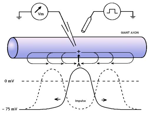
FIG 6 The impulse in the squid axon. The impulse has been
triggered by a brief depolarization at A. Note that the impulse has the ability
to spread in both directions when elicited experimentally in the middle of a
nerve.
The diameter of axons varies from 1μm to 25 μm in
humans. Axons with small diameter could be non-myelinated. However the larger
axons are ensheathed by multiple membrane layers known as myelin. In the central
nervous system (CNS) the myelin is produced by supportive glial cells called
oligodendrocytes. The oligodendrocytic membrane rotates around the axon and
forms a multiple-layered phospholipid structure that insulates the axon from the
surrounding environment. One axon is insulated by numerous oligodendrocytes
abreast, each ensheating a short segment only. Yet between two successive
oligodendrocytes tiny places remain where the axonal membrane is non-myelinated.
Between the embracing membranes of different oligodendrocytes, therefore, the
axonal membrane presents such places free of myelin. They are called nodes of
Ranvier and are enriched in voltage-gated ion channels.
In the peripheral nervous system (PNS) the myelin is
produced not by oligodendrocytes but by Schwann cells. The main principles
governing the electric behavior of axons however remain the same.
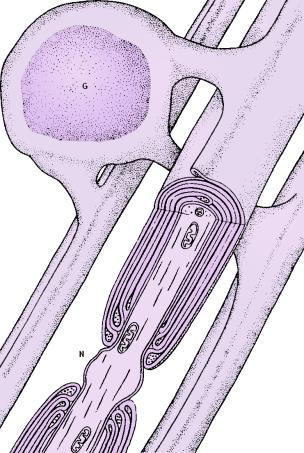
FIG
7
Oligodendrocytic glial
projections wrap three axons in CNS forming multilamelar myelin envelopes. One
oligodendrocyte typically supports 30-40 myelinated segments of different axons
in the way indicated on the diagram. Legend: G, oligodendrocytic glial cell; N,
node of Ranvier.
In the myelinated axons the membrane conductivity for ions
is substantially decreased by the multiple glial wrappings around the axon in
the form of myelin. Since the myelin sheath is not permeable for ions, the ion
leakage across the membrane is prevented and thus the axonal space constant λ
is increased. The increment of λ means that the passive spread of
voltage along the axon does not decrement so fast – and the length of axon in
which the voltage stands over the threshold is greater. This allows farther
parts of axonal membrane to become activated, thereby increasing the conducting
velocity of the action potential. In the myelinated axons the spike (action
potential) does not propagate smoothly, therefore: it jumps from node to node of
Ranvier. This is why the propagation of the action potential is called saltatory
conduction.
Saltatory conduction is made very effective and economic
because the sodium and potassium channels are clustered at the Ranvier nodes
only. This allows such neurons, possessed with less synthesized proteins (ion
channels) but more properly distributed, to achieve effective communication via
electric signals. On the other hand the passive spread of voltage remains
several orders of magnitude faster that the conducting velocity of the action
potential; myelinated neurons wisely invented the mechanism to increase the
conducting velocity of axonal spikes by way of increasing λ
– allowing only passive electric processes in the regions between two Ranvier
nodes.

FIG 8 Axonal spike in myelinated neuron generated by sodium
and potassium ion currents across the membrane in the nodes of Ranvier.
Higher stimulus intensity upon the nerve cell is thus
reflected in increased frequency of impulses, not in higher voltages because all
action potentials look essentially the same. The speed of propagation of the
action potential for mammalian motor neurons is 10-120 m/s; while for
unmyelinated sensory neurons it's about 5-25 m/s. (Unmyelinated neurons fire in
a continuous fashion, i.e. without the jumps, but the ion leakage slows the rate
of propagation).
Usually one thinks that in dendrites the passive spread of
voltage is the only mechanism that allows for effective dendritic computation.
Experimental evidence disproves this common belief. Molecular studies via
different types of labeling procedures have indeed shown that dendrites
posses voltage-gated ion channels, and that these channels are located in
domains – the so-called “hot spots”.
Although the dendritic membrane is unmyelinated, the ion
channel distribution on it is inhomogeneous. The dendritic ion channels are
clustered at (i) the postsynaptic membrane, (ii) the dendritic spine heads and
(iii) the places of dendritic branching. This particular clustering is supported
by anchoring of the voltage gated ion channels to components of the cytoskeleton
and also by incorporating the ion channels into rigid highly specialized domains
of the membrane, known as lipid rafts.
Lipid rafts are subdomains of the plasma membrane that
contain high concentrations of cholesterol and glycosphingolipids. While the
rafts exhibit a distinctive protein and lipid composition differing from the
rest of the membrane, all rafts do not appear to be identical in terms of the
proteins or the lipids that they contain. Indeed several types of lipid rafts
were found to exist, some of which are highly specific for neurons. It thus
seems that lipid rafts introduce order in the membrane, which initially was
thought as if it were highly fluid and chaotic (Linda
J. Pike, 2003). Recent advances in lipidology show both heterogeneity
of the membrane component distribution as well as the formation of organized
membrane domains in the form of rafts. As considered below, the clustering of
voltage gated ion channels and their heterogeneous distribution allow dendrites
to implement different computational gates such as AND, OR, and NOT.
The next diagram summarizes the three types of active
spread of potentials: (i) in unmyelinated axons, (ii) in myelinated axons and
(iii) in dendritic trees.
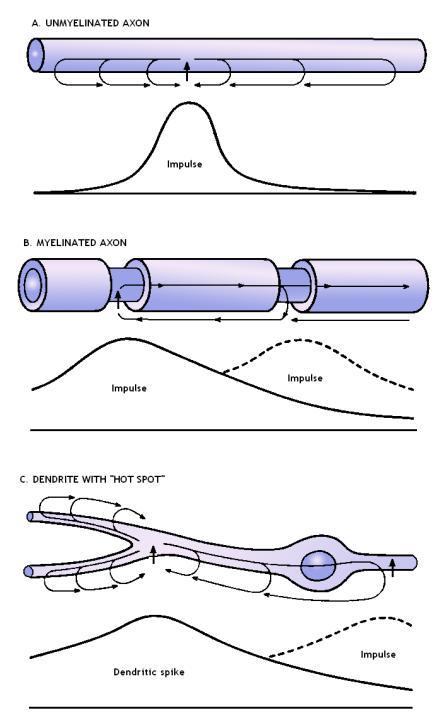
FIG
9 Comparative
image of the mechanisms
for spread of the impulse. A. Continuous conduction in an unmyelinated axon.
Amplitude scale is in millivolts. B. Discontinuous (saltatory) conduction from
node to node in a myelinated axon. C. Discontinuous spread from "hot
spot" to "hot spot" in a dendrite. In all diagrams, the impulses
are shown in their spatial extent along the fiber at an instant of time. The
extent of current spread is governed by the cable properties of the fiber.
The main communication between two neurons is achieved via
axo-dendritic synapses located at the top of the dendritic spines that are
typical for the cortical neurons. It is known that the dendritic postsynaptic
membranes convert the neuromediator signal into postsynaptic electric current.
The neuromediator molecules bind to specific postsynaptic ion channels and open
their gates. The ion species that enter the dendritic cytoplasm then change the
membrane potential.
In this section we will calculate the electric intensity
![]() in the dendritic protoplasm as well
as the magnetic flux density
in the dendritic protoplasm as well
as the magnetic flux density
![]() born by the cytoplasmatic electric
currents. In our calculations we will consider only the postsynaptic potentials
evoked by a neurotransmitter and will use the passive cable equation for
dendrites. However we should remember that
born by the cytoplasmatic electric
currents. In our calculations we will consider only the postsynaptic potentials
evoked by a neurotransmitter and will use the passive cable equation for
dendrites. However we should remember that
(i)
the action potentials generated at the axonal
hillock exhibit passive electric properties and lead to a decrementing in
space-time, retrograde (also called antidromic) rise of the electric field in
the basal dendrites and the neuronal soma;
(ii)
some action potentials generated at the axonal
hillock propagate retrogradely, because of the voltage gated sodium and calcium
channels in dendrites.
Sayer et al. (1990)
measured the evoked excitatory postsynaptic potentials (EPSP) by single firing
of the presynaptic terminal. In their study 71 unitary EPSPs evoked in CA1
pyramidal neurons (CA means Cornus Ammonis, or hippocampus) by activation of
single CA3 pyramidal neurons were recorded. The peak amplitudes of these EPSPs
ranged from 0.03 to 0.665 mV with a mean of 0.131 mV. Recently it become clear
that the remote synapses produce higher EPSPs or in other words they “speak
louder” than the proximal synapses because of voltage-gated sodium channel
boosting (Spruston,
2000) – so that the somatic EPSP amplitude is independent of
synapse location in hippocampal pyramidal neurons (Magee
& Cook, 2000). In the calculations carried out in this paper we
will consider that the single EPSP magnitude is 0.2mV (London & Segev, 2001).
Before we calculate the electric field intensity
![]() in the dendritic cytoplasm we
should assess the values of the time and space constants in the cable equation.
in the dendritic cytoplasm we
should assess the values of the time and space constants in the cable equation.
In vivo the time constant τ
depends on the membrane resistance Rm. It changes in time because the
membrane channels close and open; i.e. in vivo the membrane is active, not a
passive device. It was experimentally shown that the resistivity of the
dendritic membrane follows a sigmoid function (Waldrop
& Glantz, 1985). Its time constant τ depends on the channel conductances (Mayer & Vyklicky, 1989) and if directly calculated we
obtain a wide range of results, from 10 ms to 100 ms. The change in time of the
electric properties of neuronal membranes leads to a non-linear behavior of the
neuronal projections – and as we saw because these processes must be fueled
with energy they are labelled as active processes. All these things considered,
if interested in
the passive membrane properties
we could approximate τ
as constant in time and take τ = 30 ms.
The space constant λ
depends on the geometry of the neuronal projection and particularly on its
diameter. The space constant λ for a dendrite with d = 1μm is:
Here it should be mentioned that the space constant λ
depends on the dendrite’s diameter. So in order to be more precise in our
calculations we must decompose the dendritic tree into smaller segments with
approximately the same λ (Sajda,
2002).

FIG 10 Cable net approximation of the dendritic tree.
But if we need only a rough approximation we could consider
that the dendrite has a constant diameter of 1μm and we can use the
calculated value for the space constant, namely putting λ
= 353 μm.
On the graphics below it is presented the distribution in
space and time of a single EPSP with magnitude 0.2mV applied at the top of such
dendritic projection.

FIG 11 Spatio-temporal decrement of a single EPSP in time
interval of 40 ms in dendrite with diameter d = 1 μm, length l = 1 mm,
space constant λ
= 353 μm and time constant τ = 30 ms.
The maximal electric field intensity for a single
excitatory postsynaptic potential with magnitude 0.2 mV is
![]() = 0.57 V/m.
= 0.57 V/m.

FIG
12 Distribution of the electric intensity along the axis of the
dendrite after application of single EPSP with magnitude of 0.2 mV at the top of
a single dendrite with diameter d = 1 μm, length l = 1 mm, time interval of
40 ms, λ = 353 μm and τ
= 30 ms.
Considering that the excitatory
postsynaptic potentials (EPSPs) and the inhibitory postsynaptic potentials
(IPSPs) could summate over space and time, it is not a surprise that, in case of
multiple dendritic inputs, the measured axial dendritic voltages reach tens of
millivolts. If 300 or 400 EPSPs get temporally and spatially summated, the
electric intensity along the dendritic axis could thus be as high as 10 V/m in
different regions of the dendritic tree. The accuracy of our calculations is
supported by Jaffe & Nuccitelli (1977) who estimate the
intracellular electric fields in vivo to have intensity of 1-10 V/m.
Calculation of electric current along the dendrite after an
EPSP with magnitude of 0.2 mV gives us:
This result is smaller than the registered evoked
inhibitory postsynaptic currents (eIPSCs), whose amplitude varies from 20 pA to
100 pA (Kirischuk et al., 1999; Akaike
et al., 2002; Akaike & Moorhouse, 2003).
The mean current density J through the cross section of the
neuronal projection could be calculated from:
The above calculation is valid for a single EPSP with
amplitude of 0.2 mV. We should remind, too, that it yields mean current density
(i.e. averaged one) since the current density decrements in space exactly as the
voltage does.
The distribution of the magnetic intensity
![]() inside the projection (cable) and
outside it offers a different picture. This is so because inside the cable
inside the projection (cable) and
outside it offers a different picture. This is so because inside the cable
![]() depends on the partial interweaved
current
ix
, while outside the cable the whole current is already inside the
depends on the partial interweaved
current
ix
, while outside the cable the whole current is already inside the
![]() loop. The magnetic intensity
loop. The magnetic intensity
![]() outside the cable is
outside the cable is
![]()
where
i
is the current in the cable and x
is the distance from the axis of the cable.
The magnetic intensity inside the cable depends on the
partial interweaved current
ix
, so in case with constant current density J we can write
![]()

FIG 13 Transversal slice of a cable with radius R and
distribution of the magnetic intensity inside the cable and outside it. Legend:
H, magnetic intensity; R, cable radius; 1, area inside the cable; 2, area
outside the cable; x, distance from the cable axis. Modified from Zlatev
(1972).
The current inside dendrites is experimentally measured to
be from 20 pA to 100 pA for GABAergic synapses (Akaike
& Moorhouse, 2003). Using the formula:
![]()
we can find the magnetic intensity for a contour Γ
with length l
= πd that
interweaves the whole current ia. For dendrite with d = 1μm we
obtain:
If we consider that the water and the microtubules form a
system augmenting the magnetic strength known as ferrofluid (Frick
et al., 2003; Ávila & Funes, 1980) then in the
best-case with effective magnetic permeability μeff~10, where

we will obtain the maximal possible magnitude of the
magnetic flux density
![]() inside the neuronal projection:
inside the neuronal projection:
We should warn however that this maximal magnetic flux
density
![]() is just beneath the dendritic
membrane, and in a point of the dendritic axis the magnetic flux density is
average on the biologically relevant scales is zero. On microphysical scales it
is not zero, of course; the quantum vacuum’s “popping out” of photons
generates huge yet quasi-local values.
is just beneath the dendritic
membrane, and in a point of the dendritic axis the magnetic flux density is
average on the biologically relevant scales is zero. On microphysical scales it
is not zero, of course; the quantum vacuum’s “popping out” of photons
generates huge yet quasi-local values.
The Earth’s magnetic field is on the order of ½ Gauss (5×10⁻⁵
T). Gauss is a unit used for small fields like the Earth’s magnetic field and
1 Gauss is 10-4 T. It is thus obvious that the magnetic field
generated by the dendritic currents cannot be used as informational signal
because the noise resulting from the Earth’s magnetic field will suffocate it
(Georgiev, 2003). Or in other words any
putative magnetic signal inside the neuronal network will be like a “butterfly
in a hurricane”. This is why the magnetic field cannot encode information and
be used in the informational processing performed by neurons.
After the neuromediator molecules bind to postsynaptic ion
channel receptors, the latter open their pores. A flux of ions is thus usually
triggered across the membrane. The translocation of these ions changes the
transmembrane potential, V, and the applied voltage V spreads passively toward
the spine stalk, nearby spines and the supporting dendrite. Biological data however show that both the spine heads
as well as the “hot spots” or patches of the dendritic
membranes enriched with voltage sensitive channels, can amplify or process the
postsynaptic potentials (PSPs) via non-linear response.
In an intracellular study of hippocampal neurons Spencer & Kandel (1961) described fast prepotentials
(FPPs), small potential steps immediately preceding full-blown spikes. They
concluded that the FPPs were also spikes because of their all-or-none character
and because their repolarization was faster than the membrane time constant. In
their discussion, Spencer & Kandel (1961) proposed that
FPPs were distant dendritic spikes produced in a “trigger zone,” presumably
associated with a bifurcation of the apical dendrite. Although conceptually
influential, prepotentials did not furnish unambiguous experimental evidence for
active dendrites (Yuste & Tank, 1996). Nevertheless, in a
series of seminal papers Llinas and collaborators ushered in a new era in
dendritic physiology by recording intracellularly from dendrites of Purkinje
neurons, directly demonstrating the existence of dendritic spikes (Llinas & Nicholson, 1971; Llinas
& Hess, 1976; Llinas & Sugimori, 1980).
The dendritic spine consists of a spine head (where the
synapse gets formed) and spine stalk (a narrowing of the spine diameter that
raises the stalk resistance up to 800 MΩ (Miller
et al., 1985). Based upon the assumption that spine head membrane is
passive, previous studies concluded that the efficacy of a synapse onto a spine
head would be less than or equal to the efficacy of an identical synapse
directly onto the “parent” dendrite (Chang, 1952; Diamond et al., 1970; Coss
& Globus, 1978). However, for an active spine head membrane,
early steady state considerations suggested that spines might act as synaptic
amplifiers (Miller et al., 1985). This means that the ion channels located
in the spine head are voltage-gated and the EPSP propagation will exhibit
non-linear properties. When the voltage in the spine reaches certain voltage
magnitude (threshold) the channels open and amplify the synaptic input.
In the cerebral cortex, about 90% of the synapses are on
spines of dendritic trunks and branches. It thus may be assumed that the
dendritic microcircuits provide the main substrate for synaptic interactions.
Since much of this dendritic substrate is remote from the cell body, our
knowledge of the basic properties involved is limited. Information, nonetheless,
has been obtained by recording intracellularly from dendrites in isolated
cortical slices (Shepherd, 1994). These experiments supported
previous evidence suggesting that the cortical dendrites, like those of many
other types of neurons, harbor ionic membrane channels that are voltage
sensitive. It has been believed that these sites are located at the branch
points, where they would serve to boost the responses of distal dendrites.
The ubiquitousness of voltage-dependent channels suggested
that they may also be present in spines. The way that their presence would
contribute to spine responses and spine interactions has been explored in
computer simulations. A simulation consists in representing some portion of a
dendritic tree with its spines by means of a system of compartments – each
compartment comprising the electrical properties of a dendritic segment or
spine. It was shown that an active response in a spine would indeed boost the
amplitude of the synaptic response spreading out of the spine. It was further
shown that the current spreading passively out of one spine readily enters
neighboring spines, where in turn it can trigger further active responses. In
this way, it is thought, distal responses can be brought much closer to the cell
body by a process resembling saltatory conduction in axons.
A third interesting property is that the interactions
between active spines can be readily characterized in terms of logic operations (Shepherd & Brayton, 1987). Thus, an AND operation is
performed when two spines must be synaptically activated simultaneously in order
to generate spine responses. An OR operation is performed when either one spine
or another can be activated by a synaptic input. Finally, a NOT-AND operation
occurs when a response can be generated by an excitatory synapse if an
inhibitory synapse is simultaneously active. The interest of these simulations
is that these three logic operations, together with a level of background
activity, are sufficient for building a computer.
This result of course does not mean that the cortex is a
computer; rather, it helps to define more clearly the nature of the synaptic
interactions that take place at the microcircuit level. Defining these
interactions more clearly is a step toward identifying the basic operations
underlying the higher levels functions of circuit organization. One can
speculate that interactions of this nature within dendrites may serve the bodily
operations at play both in our outer behavior and higher cognitive functions such
as logical and abstract reasoning.
In the last several years there was extensive study of
dendritic spine active properties and a lot of experiments mapped the
distribution of the voltage-gated ion channels. At the present time it seems
that cortical neurons are the best candidates for neurons performing active
computation at the level of dendritic spines. On the next table we present the
specific distribution of voltage gated ion channels in the apical and basal
dendrites of a typical cortical neuron - the hippocampal CA1 neuron.
Table 3
Distribution
of ion channels in the dendritic tree of a CA1 hippocampal neuron. Data obtained
by Neuron
DB. The channel names are updated according to The
IUPHAR Compendium of Voltage-gated Ion Channels released in 2002.
|
Distal
apical dendrite |
Middle
apical dendrite |
Proximal
apical dendrite |
Distal
basal dendrite |
Middle basal dendrite |
Proximal
basal dendrite |
|
Cav2.2 |
Cav2.2 |
Kv1.1 Kv1.2 Kv1.6 |
KCa1.1 KCa2.1 KCa2.2 |
Nav1.x |
Nav1.x |
|
Kv3.3 Kv3.4 Kv4.1 Kv4.2 Kv4.3 |
Kv1.1 Kv1.2 Kv1.6 |
Nav1.x |
|
|
|
|
Cav2.1 Cav2.3 |
Cav2.1 Cav2.3 |
Cav2.1 Cav2.3 |
|
|
|
|
Cav3.1 Cav3.2 Cav3.3 |
Nav1.x |
Cav3.1 Cav3.2 Cav3.3 |
|
|
|
|
Nav1.x |
Cav3.1 Cav3.2 Cav3.3 |
Cav1.2 Cav1.3 |
|
|
|
|
Cav1.2 Cav1.3 |
Cav1.2 Cav1.3 |
Cav2.2 |
|
|
|
|
HCN1 HCN2 HCN3 |
Kv3.3 Kv3.4 Kv4.1 Kv4.2 Kv4.3 |
Kv3.3 Kv3.4 Kv4.1 Kv4.2 Kv4.3 |
|
|
|
|
|
HCN1 HCN2 HCN3 |
HCN1 HCN2 HCN3 |
|
|
|
According to the IUPHAR
nomenclature the name of an individual channel consists of the chemical symbol
of the principal permeating ion (e.g. Na) with the principal physiological
regulator (e.g. voltage) indicated as a subscript (e.g. Nav). The
number following the subscript indicates the gene subfamily (e.g. Nav1),
and the number following the full point identifies the specific channel isoform
(e.g. Nav1.1). This last number has been assigned according to the
approximate order in which each gene was identified. Splice variants of each
family member are identified by lower-case letters following the numbers (e.g.
Nav1.1a).
The abbreviation Nav1.x denotes all nine types
of voltage gated sodium channels from Nav1.1 to Nav1.9.
Sodium impulses may underly fast prepotentials that boost distal EPSPs. Lipowsky et al. (1996) experimentally verified that the
dendritic Na+ channels amplify EPSPs in hippocampal CA1 pyramidal
cells. Na+ action potentials support backpropagating impulses and can
activate Ca2+ action potentials (Spruston
et al., 1995). Patch recordings yield an approximate channel density
of 28 pS/micron2 in juvenile rats, which were 4 weeks of age, rising
to 61 pS/micron2 in older rats. Channel density was similar in other
dendritic compartments (Magee & Johnston, 1995; Tsubokawa
et al., 2000). Caldwell
et al. (2000) showed with immunofluorescent mapping that Nav1.6
channels are localized not only in axons and nodes of Ranvier but also in
dendrites of cortical neurons.
Recordings using the intracellular perfusion method showed
no differences between the I-V characteristics of CA1 and CA3 neurones for this
current. In contrast to this, the steady-state inactivation of both types of
neurones was significantly different (Steinhauser
et al., 1990). Inactivation of the dendritic Na+ channel
contributes to the attenuation of activity-dependent backpropagation of action
potentials (Jung
et al., 1997). Slow inactivation of sodium channels in dendrites and
soma will modulate neuronal excitability in a way that depends, in a complicated
manner, on the resting potential and previous history of action potential firing
(Mickus et al., 1999). Dendrites can fire sodium
spikes that can precede somatic action potentials, the probability and amplitude
of which depend on previous synaptic and firing history. Some dendritic spikes
could occur in the absence of somatic action potentials, indicating that their
propagation to soma is unreliable (Golding & Spruston, 1998).
Single action potential backpropagations show a dichotomy
of either strong attenuation (26-42%) or weak attenuation (71-87%). The
dichotomy seems primarily conferred by differences in distribution and density
of the voltage dependent sodium and potassium channel (A-type, especially)
along the somatodendritic axis (Golding et al., 2001).
These two channels are also known as L-type Ca2+
channels or high voltage-activated, large conductance (HVA1) channels. Using a
monoclonal antibody Westenbroek et al., (1990) showed that the
proximal dendrites and somata of hippocampal neurons label for L-type Ca2+
channels and that these channels tend to cluster near the bases of the neural
processes. In dendrite-attached patch-clamp recordings L-type channels were
occasionally encountered primarily in the more proximal dendrites – and in the
soma (Magee & Johnston, 1995). Ca2+
fluorescence imaging shows that application of L-channel antagonists reduces the
Ca2+ influx associated with backpropagating action potentials, and
has a significantly greater effect in the proximal dendrites than in more distal
dendrites (Christie, 1995).
Cav2.1 is known as P/Q-type Ca2+
channel and Cav2.3 as R-type Ca2+ channel. Dendrite-attached
patch-clamp techniques from the apical dendrites (up to 350 μm away from
soma) of CA1 pyramidal neurons in rat hippocampal slices indicate channels
similar in their basic characteristics to one or more of the high
voltage-activated, moderate conductance (HVAm) channel types (most likely P/Q-
or R-type channels)(Magee & Johnston, 1995). Ca2+
fluorescence imaging shows that application of P-channel antagonists reduces the
Ca2+ influx associated with backpropagating action potentials. Action
potential-mediated depolarization can result in the elevation of dendritic
intracellular Ca2+ concentration (Jaffe,
D.B. et al, 1992), which is important for the induction of long-term
changes in synaptic strength (Spruston
et al., 1995).
Also known as N-type Ca2+ channels. Ca2+
fluorescence imaging shows that application of N-channel antagonists slightly
reduces the Ca2+ influx associated with backpropagating action
potentials (Christie, 1995). With the use of confocal
microscopy these channels were found to be localized on the soma,
dendrites, and a subpopulation of dendritic spines (Mills
et al., 1994).
These 3 channels are also known as T-type Ca2+
channels. Patch recordings yield in dendrites an approximate channel density of
7 pS/micron2 in juvenile rats, which were 4 weeks of age – rising
to 10 pS/micron2 in older rats. T-type channels are less dense in the
soma than in the dendrites (Magee
& Johnston, 1995). Ca2+ channel density was similar in
other dendritic compartments, and in general lower than Na+ channel
density (Magee & Johnston, 1995). However, in a few apical patches
the channel density was increased three-fold, which could indicate channel
clustering. Ca2+ fluorescence imaging shows that application of
T-channel antagonists reduces the Ca2+ influx associated with
backpropagating action potentials, and has a twofold greater effect in the soma
than in the dendrites (Christie, 1995).
These channels are also known as delayed rectifiers or
D-type K+ channels, because are sensitive to dendrotoxin (DTX). A
D-type potassium current is involved in dendritic calcium spikes initiation and
repolarization (Golding et al, 1999).
These channels, also called A-type K+ channels,
are responsible for the IA current. Patch-clamp recordings reveal a
high density of A-type K+ channels in the dendritic tree, which
increases with the distance from the soma (Hoffman
et al., 1997). A shift toward more depolarized potentials of the
activation curve has also been observed in mid and distal dendrites (more than
100μm) (Hoffman
et al., 1997). These channels prevent initiation of an action
potential in the dendrites, limit the backpropagation of action potentials into
the dendrites, and reduce excitatory synaptic events (Hoffman
et al., 1997). Single action potential backpropagations show a
dichotomy of either strong attenuation (26-42%) or weak attenuation (71-87%).
The dichotomy seems to be primarily conferred by differences in distribution,
density, etc. of voltage dependent sodium and potassium channel (A-type,
especially) along the somatodendritic axis (Golding et al., 2001).
In the hippocampus, CA1 neurons and subicular neurons
differ in firing pattern (the former being regular and the later being either
regular, weakly bursting or strongly bursting) and resting membrane properties
(such as input resistance and membrane time constant); however, in both regions
a low concentration of 4-AP can convert neurons into firing bursting action
potentials (Staff et al., 2000).
KCa1.1 is known as BK channel, KCa2.1
is known as SK1 channel and KCa2.2 as SK2 channel. A single-electrode
voltage-clamp technique was employed on slices to examine slow
after-hyperpolarization (sAHP). This was achieved by using conventional
procedures to evoke an after-hyperpolarization (AHP) in the current clamp,
rapidly followed by a switch into voltage clamp (hybrid clamp). The AHP current
showed a dependence on extracellular K+ close to that predicted by
the Nernst equation. It could be blocked by Cd2+ or norepinephrine
and showed a requirement for voltage-dependent Ca2+ entry, but did
not show any clear intrinsic voltage dependence. Once activated, AHP current is
not turned off by hyperpolarizing the membrane potential (Lancaster & Adams, 1986). Cell-attached patches on the
proximal 100 μm of the apical dendrite did not contain sAHP channels.
Amputation of the apical dendrite approximately 30 μm from the soma, while
simultaneously recording the slow AHP whole cell current at the soma, depressed
the sAHP amplitude by only approximately 30% compared with controls. Somatic
cell-attached and nucleated patches did not contain sAHP current. Amputation of
the axon about 20 μm from the soma had little effect on the amplitude of
the slow AHP. By this process of elimination, it is suggested that the sAHP
channels may be concentrated in the basal dendrites of CA1 pyramids (Bekkers,
2000).
In situ hybridization showed high levels of expression of
SK1 and SK2 channels in CA1-3 regions of the hippocampus (Stocker & Pedarzani, 2000). The role of large-conductance
Ca2+-dependent K+ channels (BK) in spike broadening during
repetitive firing was studied by using sharp electrodes and by computer
modelling. The amplitude of the fast after-hyperpolarization (fAHP) rapidly
declined during each train. Suppression of BK-channel activity with the
selective BK-channel blocker iberiotoxin, the non-peptidergic BK-channel blocker
paxilline, or calcium-free medium, broadened the first spike to a similar
degree, of approximately 60 %. (Shao, L.R. et al., 1999).
These channels, also called hyperpolarization-activated,
cyclic nucleotide-gated cation channels, are responsible for the Ih current. A
depolarizing lag during larger hyperpolarizing voltage transients is indicative
of Ih current in CA1 pyramidal neurons (Spruston
& Johnston, 1992). Membrane patches recorded in the cell-attached
patch configuration from the soma and apical dendrites revealed an Ih that
increased over six-fold from soma to distal dendrites. Ih demonstrated a mixed
Na+-K+ conductance and was sensitive to low concentrations
of external CsCl. As a result of Ih the propagation of subthreshold voltage
transients is directionally specific. The elevated dendritic Ih density
decreases EPSP amplitude and duration and reduces the time window over which
temporal summation takes place (Magee, 1999).
From the computational point of view, the neuronal soma
integrates the inputs from the dendrites. The passive properties of dendrites
lead to decrement of the EPSPs and IPSPs that reach the soma. This however
allows for the EPSPs and IPSPs to summate over space and time – and when a
critical threshold in the soma is reached a non-decrementing axonal spike to
occur.
The nonlinear properties of the neuronal output are due to
voltage-gated Na+ channels located at the axon hillock
that exhibit positive feedback. When a critical threshold of the transmembrane
voltage of about -55mV is reached in the axonal hillock, more and more
voltage gated sodium ion channels get open and an action potential is triggered.
The magnetic and the electric field strengths are expected to be the same as in
the axon, with maximal magnetic strength of 10-7 T and maximal
electric strength of 10 V/m (see below).

FIG 14 Standard model of informational processing. Inputs from
other neurons are multiplied by the corresponding passive dendritic weights
ω1-ω4, summed (Σ) and then passed through nonlinearity.
When the voltage change in the axonal hillock reaches a
threshold potential of -55mV, action potential is triggered. The membrane
becomes depolarized due to gate opening of voltage sensitive Na+
channels, which allow Na+ to rush into cell. This is an all-or-none
event – it ineluctably happens once threshold is reached. When the inside of
membrane is depolarized to +40mV, Na+ gates shut and K+
gates open. K+ rushes out trough the open K+ gates while
the Na+ gates are closed and inactive. The membrane thus becomes
repolarized and may even get hyperpolarized. Refractory period occurs while the
Na+ gates of Na+ channels remain closed:
the membrane will not respond again until Na+ gates become
active.
The electric current flow across the cell membrane depends
on the capacitance of the membrane and the resistance of the ion channels. The
total ionic current is represented by the sum of the sodium current, potassium
current and a small leakage current. The leakage current represents the
collective contribution of ions such as chloride and bicarbonate.
The Hodgkin-Huxley model represents an isopotential
membrane patch or a single electrical compartment, i.e., there are no spatial
effects on the potential (Hodgkin & Huxley, 1952a; 1952b; 1952c; 1952d;
1952e; 1952f). The units of the model are per
membrane unit area, whence it is then straightforward to scale the model to a
single compartment of any desired membrane area.
The total membrane current is the sum of the ionic currents
and the capacitive current
where Im is the membrane current density, Iionic
are the ionic currents densities, CM is the membrane capacity per
unit area and Vm is the membrane voltage. The two main ionic
conductances, sodium and potassium are independent of each other, and a third,
leak conductance does not depend on any of the other conductances or the
membranal voltage. Thus, the total ionic current is the sum of the separate
ionic currents.

FIG 15 An electrical circuit diagram describing the current
flows across the cell membrane that are captured in the Hodgkin-Huxley model.
Compare with Fig. 5.
The individual ionic currents are linearly related to the
potential according to Ohm’s law,
where GK, GNa and GL are
the potassium, sodium and leak conductances per unit area of the membrane and EK,
ENa and EL are the corresponding reversal or equilibrium
Nernst potentials of each of the ionic species.
The voltage-dependent conductances GNa(t) and
GK(t) are given by
where
![]() and
and
![]() are the peak or maximal sodium and
potassium conductances per unit membrane area and fNa(t) and fK(t)
are each the corresponding (instantaneous) fraction of the maximal conductance
which is actually open (or active). Thus the equation, which describes the
membrane potential as a function of all the currents that flow across it, is
are the peak or maximal sodium and
potassium conductances per unit membrane area and fNa(t) and fK(t)
are each the corresponding (instantaneous) fraction of the maximal conductance
which is actually open (or active). Thus the equation, which describes the
membrane potential as a function of all the currents that flow across it, is
The
values for some of the parameters are: ENa= +60 mV,
![]() = 120 mS/cm2, EK= -93 mV,
= 120 mS/cm2, EK= -93 mV,
![]() = 36 mS/cm2, EL= -60 mV and
= 36 mS/cm2, EL= -60 mV and
![]() = 0.3 mS/cm2.
= 0.3 mS/cm2.
The Hodgkin-Huxley model replicates many of the features of
spiking of the squid giant axon: the form, duration and amplitude of a single
spike (both for the membrane and the propagating spike), its sharp threshold,
the conduction velocity of the spike along the axon, the refractory period of
the neuron, the impedance changes during the spike, anode-break excitation,
accommodation, subthreshold response and oscillations. When simulating the
response to sustained stimulus currents, it demonstrates a discontinuous onset
of repetitive firing with a high spiking frequency and a limited bandwidth of
the firing frequency.
However, careful studies of the model reveal that it does
not provide a good description of quite a few electrophysiological properties of
the axon (Clay, 1998), in particular the refractory behavior of the
preparation in response either to sustained or periodic current pulse
stimulation. Also, the model does not account for after potentials and slow
changes in the squid giant axon.
Still, the Hodgkin-Huxley model serves as the golden
standard of neuronal excitability, and with minor changes - as the backbone of
most neuronal spiking models. The main reason is that the Hodgkin-Huxley model
does capture the essence of spiking through ionic currents (Na+ and K+),
which enter and leave the cell through voltage dependent channels. Moreover, the
model is compact, and approximates well many of the features shared by different
types of neurons (shape and duration of spiking, repetitive spiking in response
to sustained inputs, refractoriness, etc.) while incorporating biophysical
aspects of the neuron. Adding the appropriate currents for other channel types
(usually using similar kinetic schemes) is easily done. Accordingly, and since
the model has been studied mathematically in great detail (Jack et al., 1975), it is the common choice of
conductance based modeling for computational studies and theoretical ones.
In this section we will pay attention once more on the fact
that in every neuronal electric process both active and passive events are
involved. The passive spread of the electric currents and electric field happens
very fast. These processes can be well described if we take the membrane
resistance and capacitance as constant in time. In contrast, the active
processes rely on changes in membrane conductivity via gating of ion channels
sensitive to voltage.
The action potential generated at the axonal hillock
propagates down the axon because of the opening of voltage gated sodium
channels. Because the soma and nearby dendrites lack proper distribution of
voltage gated ion channels, the action potential does not propagate actively in
retrograde direction – or if it does, as we have seen in the previous section
when discussing active dendritic properties, it is rare event so that the
antidromic (retrograde) propagation of the action potential helps in
establishing long-term potentiation (LTP) in dendrites. The passive spread of
electric field, however, cannot be prevented. Its depth of penetration depends
on the space constant λ, which increases with the
increase of the membrane resistance. Conversely, if the membrane resistance is
low, ionic leakage through the membrane occurs and the voltage drops faster
because λ decreases; at this point one should remember that
the space constant λ has the meaning of the distance at which the
applied voltage drops e = 2.72 times. On the next picture it is presented a
stretch-receptive neuron from crayfish, with dendrites terminating on a muscle
fiber. Both dendritic EPSP and IPSP spread are depicted, as well as the
retrograde passive spread of the action potential.
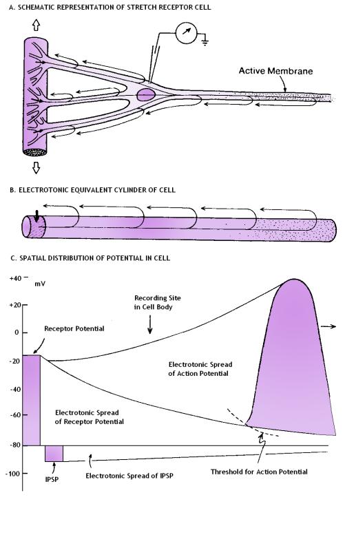
FIG 16 Stretch receptor neuron of the crayfish. The receptive
neuron has several large dendritic trunks, which enter the muscle and terminate
in fine branches. When stretch is applied to the muscle, a depolarization is set
up in the dendritic branches, graded with the amount of stretch.
It would be naïve to expect extreme electric field
intensities in the axon compared to the field intensity in dendrites. This is
because the space constant λ in axons is 1-2 orders of
magnitude larger than the dendritic space constant and λ
is inversely linked to the electric field strength
![]() . The electric field intensity could be approximated by using the cable equation
after assessing the space constant λ
for the axonal projection – that increases with the diameter of the neuronal
projection:
. The electric field intensity could be approximated by using the cable equation
after assessing the space constant λ
for the axonal projection – that increases with the diameter of the neuronal
projection:
The applied voltage during action potential is about 120 mV
(assuming that a resting membrane of -70 mV is depolarized till the potential
reaches +50 mV), so the electric field intensity
![]() is about 12 V/m.
is about 12 V/m.
The vector of the magnetic induction
![]() will form closed loops around the
axis of the neuronal projection. Their direction is defined by the right-handed
screw rule (i.e. counterclockwise if the axial current flows toward your face).
In axons the magnetic field is stronger than the magnetic field in dendrites
because of the greater ion currents flowing inside the axoplasm. The nerve
action potential has the form of a moving solitary wave, with peak currents
range from 5 to 10 µA (Katz,
B., 1966). Axons range in diameter from less than 1 μm to 25
μm in humans, but reach gigantic size in squid with d = 1mm. Calculations
of the magnetic flux density in the largest human axons that have the greatest
electric currents give us:
will form closed loops around the
axis of the neuronal projection. Their direction is defined by the right-handed
screw rule (i.e. counterclockwise if the axial current flows toward your face).
In axons the magnetic field is stronger than the magnetic field in dendrites
because of the greater ion currents flowing inside the axoplasm. The nerve
action potential has the form of a moving solitary wave, with peak currents
range from 5 to 10 µA (Katz,
B., 1966). Axons range in diameter from less than 1 μm to 25
μm in humans, but reach gigantic size in squid with d = 1mm. Calculations
of the magnetic flux density in the largest human axons that have the greatest
electric currents give us:
Although this result is 3 orders of magnitude greater than
the experimentally measured magnetic field in frog sciatic nerve using SQUID
magnetometer (Wikswo et al., 1980) it remains too weak - only 1/300
of the Earth’s magnetic field. The experimentally measured value for the
magnetic field
![]() of the frog sciatic nerve using
SQUID magnetometer was 1.2×10⁻¹⁰ T with a signal-to-noise ratio 40
to 1 (Wikswo et al., 1980). The assessed value
for magnetic field strength at the frog nerve surface (where it has peak
magnitude) using the Ampere’s law was 1.2×10⁻¹⁰ T because of large
frog sciatic the nerve diameter (d = 0.6mm).
of the frog sciatic nerve using
SQUID magnetometer was 1.2×10⁻¹⁰ T with a signal-to-noise ratio 40
to 1 (Wikswo et al., 1980). The assessed value
for magnetic field strength at the frog nerve surface (where it has peak
magnitude) using the Ampere’s law was 1.2×10⁻¹⁰ T because of large
frog sciatic the nerve diameter (d = 0.6mm).
The longitudinal electric intensity EL and the magnetic flux density in membranes are expected to be the same as the calculated values for the cytoplasm:
EL = 10 V/m
B =10-7 T
We have seen, however, that the relevant stimulus for the voltage gated ion
channels is the transmembrane voltage Vm. While its absolute values
reach V = 90 mV the intensity of the transversal electric field
ET
is tremendous because of the narrowness of the plasma membrane, which is about
10 nanometers thick. Simple calculations yield
![]()
where
h is the membrane thickness and V is the transmembrane voltage.

FIG 17 Transversal and longitudinal intensity
of the electric field in membranes.
Akaike,
N. & Moorhouse, A.J. (2003). Techniques:
Applications of the nerve-bouton preparation in neuropharmacology. Trends in
Pharmacological Sciences 24: 44-47.
Akaike, N. et al. (2002). Focal stimulation of single GABAergic presynaptic boutons on the rat hippocampal neuron. Neurosci. Res. 42: 187-195.
Alberti,
A. (1884). Contribución
al estudio de las Localizaciones Cerebrales y a la Patogénesis de la Epilepsia.
31 July 1884 Public Concourse, Círculo Médico Argentino, Buenos Aires, Ms.
Alberti,
A. (1886). Contribución al estudio de las
Localizaciones Cerebrales y a la Patogénesis de la Epilepsia. Buenos Aires,
Biedma.
Arfken,
G. (1985). "Gradient, ![]() " and "Successive
Applications of
" and "Successive
Applications of ![]() ." §1.6 and 1.9 in Mathematical Methods for Physicists, 3rd ed. Orlando,
FL: Academic Press, pp. 33-37 and 47-51.
." §1.6 and 1.9 in Mathematical Methods for Physicists, 3rd ed. Orlando,
FL: Academic Press, pp. 33-37 and 47-51.
Ávila, A. & Funes, J. (1980), Engramación por islotes de electreto:
estudio experimental de su posibilidad como mecanismo neural. Investigación #
6776, Facultad de Medicina de la Universidad de Buenos Aires; progress report in
“Guía de Invest. en curso en la Universidad de Buenos Aires vol. II”, 1984 :
Instituto Bibliotecológico de la Universidad de B. Aires.
Baker,
P.F., Hodgkin, A.L., Shaw, T.I. (1961). Replacement of
the protoplasm of a giant nerve fibre with artificial solutions. Nature 190:
885-887.
Baker, P.F., Hodgkin, A.L. & Shaw, T.I. (1962a). Replacement of the axoplasm of giant nerve fibres with artificial solutions. J Physiol. 164: 330-354.
Baker, P.F., Hodgkin, A.L. & Shaw, T.I. (1962b). The effects of changes in internal ionic concentrations on the electrical properties of perfused giant axons. J Physiol. 164: 355-374.
Baker, P.F., Hodgkin, A.L. & Meves, H. (1964). The effect of diluting the internal solution on the electrical properties of a perfused giant axon. J Physiol. 170: 541-560.
Barlaro, P. M. (lessons’ transcriber) (1909). Curso sobre enfermedades del Sistema Nervioso en relación con su Anatomía Patológica, dictado por el Dr. Chr. Jakob en la Clínica del Dr. Ramos Mejía y recogidas por el Dr. Pablo M. Barlaro, ayudante de Patología Interna. Buenos Aires, La Ciencia Médica.
Beer, B. (1902). Über das Auftrafen einer objective Lichtempfindung in magnetischen Felde. Klin. Wochenschr. 15:108-109.
Bekkers, J.M. (2000). Distribution of slow AHP channels on hippocampal CA1 pyramidal neurons. J. Neurophysiol. 83: 1756-1759.
Caldwell,
J.H., Schaller, K.L., Lasher, R.S., Peles, E. & Levinson, S.R. (2000).
Sodium channel Nav1.6 is localized at nodes of Ranvier, dendrites, and synapses.
PNAS 97(10):
5616–5620
Cauller, L. (2003). Course
in Neurophysiology. Web
source: http://www.utdallas.edu/~lcauller/
Chang, H.T. (1952). Cortical neurons with particular reference to the apical dendrites. Cold Spring Harbor Syrnp. Quant. Biol. 17: 189-202.
Christie, B.R. (1995). Different Ca2+ channels in soma and dendrites of hippocampal pyramidal neurons mediate spike-induced Ca2+ influx. J Neurophysiol. 73(6): 2553-2557.
Clay, J.R. (1998). Excitability of the squid giant axon revisited. J.Neurophysiol., 80:903-913.
Cole, K.S. & Curtis, H.J. (1939). Electric impedance of the squid giant axon during activity. Journal of General Physiology 22: 649-670.
Coss, R.G. & Globus, A. (1978). Spine stems on tectal interneurons in jewel fish are shortened by social stimulation. Science 200: 787-790.
Crocco, M. F. (1994). Alberto Alberti y el primer mapeo con electricidad ¡durante ocho meses! de un cerebro humano consciente: hazaña científica silenciada durante un siglo. Electroneurobiología 1 (3), 73-82 (September). Web source: http://electroneubio.secyt.gov.ar/general.htm
Crocco, M. & Contreras, N. (1986a). Oscuridades, enigmas, y el aporte fundamental de Ricardo Sudnik (1880/4) en el origen de la neurobiología argentina. La Semana Médica 168 # 5376 (12 March 1986).
Crocco,
M. & Contreras, N. (1986b). El contexto histórico y los descubrimientos
de Alberto Alberti en las localizaciones cerebrales. La Semana Médica 168, #
5378 (5 April 1986), 217-230.
Curtis,
H.J. & Cole, K.S. (1940). Membrane
action potentials from the squid giant axon. J. Cell. Comp. Physiol. 15: 147-157
Curtis,
H.J. & Cole, K.S. (1942). Membrane
resting and action potentials from the squid giant axon. J. Cell. Comp. Physiol. 19: 135-144.
d'Arsonval,
A. (1896) Dispositifs pour la mesure des courants
alternatifs de toutes fréquences. C. R. Soc. de Biologie (Paris) 3:450-457.
Diamond, J., Gray, E.G. & Yasargil, G.M. (1970). The function of the dendritic spines: a hypothesis. In P. Anderson and J.K.S. Jansen (Eds.), Excitatory Synaptic Mechanisms, Universitetsforlaget, Oslo, pp. 213-222.
Du
Bois-Reymond, E. (1848). Untersuchungen über thierische Elektricität, Erster
Band. Berlin: Georg Reimer. The book can be downloaded from
Max Planck Institute for the History of Science (806 pages, high resolution,
~180.24 MB).
Fleshman,
J.W., Segev, I. & Burke, R.B. (1988).
Electrotonic architecture of type-identified α-motoneurons in the cat
spinal cord. Journal of Neurophysiology 60: 60-85.
Frick,
P., Khripchenko, S., Denisov, S., Sokoloff, D. & Pinton, J.F. (2003).
Effective magnetic permeability of a turbulent fluid with macroferroparticles.
EPJ manuscript. Web
source: http://www.ens-lyon.fr/~pinton/ARTICLES/mhd_SB_EPJB.pdf
Galvani,
L. (1791). De viribus electricitatis in motu
musculari, Bologna. (Translated in english: Galvani, Luigi. Commentary
on the Effects of Electricity on Muscular Motion. Norwalk, CT, 1953. 176 pp., 4
folding plates, illus. Includes facsimile and translation of Galvani's De
viribus electricitatis in motu musculari, Bologna, 1791, plus a bibliographical
study by John F. Fulton and Madeline E. Stanton.)
Georgiev,
D. (2003). Electric and magnetic fields inside
neurons and their impact upon the cytoskeletal microtubules. Web
source: http://cogprints.org/3190/
Golding,
N.L. & Spruston, N. (1998). Dendritic
sodium spikes are variable triggers of axonal action potentials in hippocampal
CA1 pyramidal neurons. Neuron. 21: 1189-1200.
Golding,
N.L., Jung, H.Y., Mickus, T. & Spruston N. (1999).
Dendritic calcium spike initiation and repolarization are controlled by distinct
potassium channel subtypes in CA1 pyramidal neurons. J Neurosci. 19: 8789-8798.
Golding,
N.L., Kath, W.L. & Spruston N. (2001). Dichotomy
of action-potential backpropagation in CA1 pyramidal neuron dendrites. J
Neurophysiol. 86: 2998-3010.
Hodgkin,
A.L. & Huxley, A.F. (1952a). Currents
carried by the sodium and potassium ion through the membrane of the giant axon
of Loligo. J. Physiol. 116(4): 449-472.
Hodgkin,
A.L. & Huxley, A.F. (1952b). The components
of the membrane conductance in the giant axon of the Loligo. J. Physiol. 116(4):
473-496.
Hodgkin,
A.L. & Huxley, A.F. (1952c). The dual
effect of membrane potential on sodium conductance in the giant axon of Loligo.
J. Physiol. 116(4): 497-506.
Hodgkin,
A.L. & Huxley, A.F. (1952d). A quantitative
description of membrane current and its application to conduction and excitation
in nerve. J Physiol. 117(4): 500-544.
Hodgkin,
A.L. & Huxley, A.F. (1952e). Propagation of
electrical signals along giant nerve fibers. Proc R Soc Lond B Biol Sci.
140(899): 177-183.
Hodgkin,
A.L. & Huxley, A.F. (1952f). Movement of
sodium and potassium ions during nervous activity. Cold Spring Harb Symp Quant
Biol. 17: 43-52.
Hoffman,
D.A., Magee, J.C., Colbert, C.M. & Johnston, D. (1997).
K+ channel regulation of signal propagation in dendrites of
hippocampal pyramidal neurons. Nature. 387: 869-875.
The
IUPHAR Compendium of Voltage-gated Ion Channels, 2002.
Jakob,
C. (1906, 1907, 1908). “Localización del alma y de la
inteligencia”, El Libro (Buenos Aires) 1 (1906), 151; and (1907), pp. 281,
433, 553; V. 2 (1908) pp. 3, 171, 293, 537 and 695 (published on nine issues).
Jakob,
C. (1911). Vom Tierhirn zum Menschenhirn, I Teil:
Tafelwerk nebst Einführung in die Geschichte der Hirnrinde. J. F. Lehmann’s
Verlag, München.
Jack,
J.J.B., Noble, D. & Tsien, R. (1975). Electric
current flow in excitable cells. Oxford.
Jaffe,
D.B., Johnston, D., Lasser-Ross, N., Lisman, J.E., Miyakawa, H. & Ross, W.N.
(1992). The spread of Na+ spikes determines the
pattern of dendritic Ca2+ entry into hippocampal neurons. Nature.
357: 244-246.
Jaffe,
L.F. & Nuccitelli, R. (1977). Electrical
controls of development. Annual Review of Biophysics and Bioengineering 6:
445-476.
Jung,
H.Y., Mickus, T. & Spruston, N. (1997). Prolonged
sodium channel inactivation contributes to dendritic action potential
attenuation in hippocampal pyramidal neurons. J Neurosci. 17: 6639-6646.
Kaplan,
W. (1991). "The Gradient Field". §3.3 in
Advanced Calculus, 4th ed. Reading, MA: Addison-Wesley, pp. 183-185.
Katz,
B. (1966). Nerve, Muscle and Synapse. McGraw-Hilt, New
York.
Kirischuk,
S. et al. (1999). Relationship
between presynaptic calcium transients and postsynaptic currents at single
GABAergic boutons. PNAS 96: 7520-7525.
Lamacq, L. (1897). Les centres moteurs corticaux du cerveau humain déterminés d'aprés les effets de l'excitation faradique des hémisphères cérébraux de l'homme. Arch. Clin. Bordeaux 6, 11-13 (novembre).
Lancaster, B. & Adams, P.R. (1986). Calcium-dependent current generating the afterhyperpolarization of hippocampal neurons. J. Neurophysiol. 55: 1268-1282.
Lipowsky,
R., Gillessen, T. & Alzheimer, C. (1996).
Dendritic Na+ channels amplify EPSPs in hippocampal CA1 pyramidal cells. J
Neurophysiol. 76: 2181-2191.
Llinas, R. & Hess, R. (1976). Tetrodotoxin-resistant dendritic spikes in avian Purkinje cells. Proc. Natl. Acad. Sci. USA 73: 2520-2523.
Llinas,
R. & Nicholson, C. (1971). Electroresponsive
properties of dendrites and somata in alligator Purkinje cells. J. Neurophysiol.
34: 532-551.
Llinas,
R. & Sugimori, M. (1980).
Electrophysiological properties of in vitro Purkinje cell dendrites in mammalian
cerebellar slices. J. Physiol. 305: 197-213.
London,
M. & Segev, I. (2001). Synaptic scaling in
vitro and in vivo. Nature Neuroscience 4(9):
853-854.
Magee,
J.C. (1999). Dendritic Ih normalizes temporal summation
in hippocampal CA1 neurons. Nat. Neurosci. 2(9): 848.
Magee,
J.C. & Cook, E.P. (2000). Somatic
EPSP amplitude is independent of synapse location in hippocampal pyramidal
neurons. Nat Neurosci. 3(9): 895-903.
Magee,
J.C. & Johnston, D. (1995). Characterization
of single voltage-gated Na+ and Ca2+ channels in apical
dendrites of rat CA1 pyramidal neurons. J Physiol (Lond). 487: 67-90.
Matteucci,
C. (1838). Sur le courant electrique ou propre de la
grenouille; second mémoire sur l'electricité animale, faisant suite à celui
sur la torpille. Paris.
Matteucci,
C. (1840). Essai sur les phénomènes électriques
des animaux. Paris.
Matteucci,
C. (1844). Traité des phénomènes électro-physiologiques
des animaux. Paris.
Mayer,
M.L. & Vyklicky, L. Jr. (1989). Concanavalin
A selectively reduces desensitization of mammalian neuronal quisqualate
receptors. PNAS 86: 1411-1415.
Mickus,
T., Jung, H. & Spruston, N. (1999). Properties
of slow, cumulative sodium channel inactivation in rat hippocampal CA1 pyramidal
neurons. Biophys J. 76: 846-860.
Miller,
J.P. (1980). Cytoplasmic resistivity of neurons in the
lobster stomatogastric ganglion.
Miller,
J.P., Rall, W., & Rinzel, J. (1985). Synaptic
amplification by active membrane in dendritic spines. Brain Res.325: 325-330.
Mills,
L.R., Niesen, C.E., So, A.P., Carlen, P.L., Spigelman, I. & Jones, O.T. (1994).
N-type Ca2+ channels are located on somata, dendrites, and a subpopulation of
dendritic spines on live hippocampal pyramidal neurons. J Neurosci. 14:
6815-6824.
Morse,
P.M. & Feshbach, H. (1953). "The
Gradient." In Methods of Theoretical Physics, Part I. New York:
McGraw-Hill, pp. 31-32.
Nave,
C.R. (2003). HyperPhysics.
Nernst, W.H. (1888). Zur Kinetik der Lösung befindlichen Körper: Theorie der Diffusion. Z. Phys. Chem. 3: 613-37.
Nernst,
W.H. (1889). Die elektromotorische Wirksamkeit der
Ionen. Z. Phys. Chem. 4: 129-81.
Neuron
DB database is being developed by Luis N. Marenco1,
Buqing Mao1, Chiquito Crasto1, Prakash M. Nadkarni1,
Perry L. Miller1 and Gordon M. Shepherd2; 1Center
for Medical Informatics; 2Section of Neurobiology; Yale University
School of Medicine, New Haven, CT 06510. Supported by NIDCD, NASA, & NIMH
(Human Brain Project) and the National Library of Medicine's IAIMS Program.
Olhoeft,
G.R. (2003).
Electromagnetic Wave Propagation Velocity.
Petrolli,
G. (2001). Alberto Alberti, neurochirurgo ítalo-argentino.
Edizioni Stella, Nicolodi Editore, Roveretto, Italia.
Pike,
L.J. (2003). Lipid rafts: bringing order to chaos. J. Lipid Res. 44: 655-667.
Sajda, P. (2002). Computational Neural Modeling and Neuroengineering. BMEN E6480. Lecture 2: Cable Theory and Dendritic Trees. Web source: http://www.bme.columbia.edu/~sajda/bme6480/
Sayer,
R.J., Friedlander, M.J. & Redman, S.J. (1990). The
time course and amplitude of EPSPs evoked at synapses between pairs of CA3/CA1
neurons in the hippocampal slice. J. Neurosci.
10: 826-836.
Schey,
H.M. (1997). Div, Grad, Curl, and All That: An Informal
Text on Vector Calculus, 3rd ed. New York: W. W. Norton.
Shao,
L.R., Halvorsrud, R., Borg-Graham, L. & Storm, J.F. (1999).
The role of BK-type Ca2+-dependent K+ channels in spike
broadening during repetitive firing in rat hippocampal pyramidal cells. J.
Physiol. 521: 135-146.
Shepherd,
G.M. (1994). Neurobiology, Third Edition. Oxford U.
Press, New York.
Shepherd,
G.M. & Brayton, R.K. (1987). Logic
operations are properties of computer-simulated interactions between excitable
dendritic spines. Neuroscience 21(1): 151-165.
Spencer,
W.A. & Kandel, E.R. (1961). Electrophysiology
of the hippocampal neurons. IV. Fast
prepotentials. J Neurophysiol. 24: 272-285.
Spruston,
N. (2000). Distant synapses raise their voices.
Nature Neuroscience 3: 849-851.
Spruston,
N. & Johnston, D. (1992). Perforated
patch-clamp analysis of the passive membrane properties of three classes of
hippocampal neurons. J Neurophysiol. 67: 508-529.
Spruston,
N., Schiller, Y., Stuart, G. & Sakmann, B. (1995).
Activity-dependent action potential invasion and calcium
influx into hippocampal CA1 dendrites. Science. 268: 297-300.
Staff, N.P., Jung, H.Y.,
Thiagarajan, T., Yao, M. & Spruston, N. (2000).
Resting and active properties of pyramidal neurons in subiculum and CA1 of rat
hippocampus. J Neurophysiol. 84: 2398-2408.
Steinhauser, C., Tennigkeit,
M., Matthies, H. & Gundel, J. (1990). Properties of the fast
sodium channels in pyramidal neurones isolated from the CA1 and CA3 areas of the
hippocampus of postnatal rats. Pflugers Arch. 415: 756-761.
Stocker,
M. & Pedarzani, P. (2000). Differential
distribution of three Ca2+-activated K+ channel subunits,
SK1, SK2, and SK3, in the adult rat central nervous system. Mol. Cell. Neurosci. 15: 476-493.
Stoilov,
S., Rusanov, E., Mitev, D. & Genkov, D. (1985).
Biophysics. Publishing house “Medicina
i Fizkultura”, Sofia.
Tsubokawa,
H., Offermanns, S., Simon, M. & Kano, M. (2000).
Calcium-dependent persistent facilitation of spike backpropagation in the CA1
pyramidal neurons. J Neurosci. 20: 4878-4884.
von
Helmholtz, H. (1850). Über die
Fortpflanzungsgeschwindigkeit der Nervenreizung. Arch. Anat. Physiol. Wiss. Med. pp.71-73. This and the two following
references are to be soon available on Helmholtz’ multivolume Gesammelte Werke
series being published by Georg Olms Verlag of Hildesheim; web source http://www.olms.de
von
Helmholtz, H. (1852). Messungen über
Fortpflanzugsgeschwindigkeit der Reizung iun Nerven. Arch. Anat. Physiol. Wiss.
Medizin. pp.199-216
von
Helmholtz, H. (1854). Uber die geschwindigkeit
einiger vorgange in muskeln und nerve. Bericht über die zur bekanntmachung
geeigneten verhandlungen der koniglichen. Preuss Akad Wiss., Berlin. pp. 328-332
Waldrop,
B. & Glantz, R.M. (1985). Synaptic
mechanisms of a tonic EPSP in crustacean visual interneurons: analysis and
simulation. Journal of Neurophysiology 54: 636-650.
Weisstein, E.W. (2003). Gradient. Wolfram Research, Inc. Web source: http://mathworld.wolfram.com/Gradient.html
Westenbroek, R.E.,
Ahlijanian, M.K. & Catterall, W.A. (1990).
Clustering of L-type Ca2+ channels at the base of major dendrites in
hippocampal pyramidal neurons. Nature. 347: 281-284.
Wikswo, J.P., Barach, J.P. & Freeman, J.A. (1980). Magnetic Field of a Nerve Impulse: First Measurements. Science 208: 53-55. Web source: http://www.vanderbilt.edu/lsp/abstracts/wikswo-s-1980.htm
Yuste,
R. & Tank, D.W. (1996). Dendritic Integration in
Mammalian Neurons, a Century after Cajal. Neuron 16: 701-716.
Zlatev,
M.P. (1972). Theoretical Electrotechnics. Volume I. Publishing house
“Tehnika”, Sofia.
![]()
Copyright
© 2004 del autor / by the author. Esta es una investigación
de acceso público; su copia exacta y redistribución por cualquier medio están
permitidas bajo la condición de conservar esta noticia y la referencia completa
a su publicación incluyendo la URL original (ver arriba). / This is an Open
Access article: verbatim copying and redistribution of this article are
permitted in all media for any purpose, provided this notice is preserved along
with the article's full citation and original URL (above).
revista
Electroneurobiología
ISSN: 0328-0446
Croquis de este sitio - Outline of this site
Índice - Table des matières
- Inhaltsverzeichnis - Table of Contents
Some
downloadable articles and documents in this site are in PDF format (.pdf). To
view or print these articles, you must have Adobe Acrobat Reader installed. Acrobat Reader can be downloaded from
Adobe's web site free of charge by clicking here / Se recomienda mucho
leer o imprimir algunos de los trabajos mas extensos con el programa Acrobat
Reader,
que puede obtenerse gratuitamente pulsando aqui ![]()
Haga doble
"click" en el título de cualquier artículo, para leerlo ahora -
Double-click on any article to read it now:
*
SOCIOLOGÍA DE LAS NEUROCIENCIAS
¡Nuevo! "L’anthropologie
ganglionnaire, un psychovirus démasqué" (français)
Puede leer, imprimir o guardar en su disco
duro esta investigación en versión .PDF
(190 kB: recomendada) o .DOC
(76 kB).
*
ELECTRONEUROBIOLOGÍA
Efectos relativísticos en
biofísica cerebral:
Puede leer, imprimir o guardar en su disco
duro esta investigación en versión .PDF (496
kB: recomendada) o .DOC (227 kB).
MBYKYHÁPE GUARANÍME SUMARIO Y PÁRRAFOS INICIALES EN CASTELLANO SUMÁRIO EM PORTUGUÊS ABSTRAKTI SUOMEKSI
*
Diversificación
de recursos electroneurobiológicos en la evolución del sistema nervioso:
Puede leer, imprimir o guardar en su disco
duro esta investigación en versión .PDF
(733 kB: recomendada) o .DOC (406
kB).
SUMÁRIO EM
LÍNGUA PORTUGUESA SUMARIO
CASTELLANO
*
Cálculo de potenciales
dentro de las células
Calcule intensidades eléctricas y magnéticas
en cada compartimiento neuronal: "The
nervous principle: active versus passive electric processes in neurons" (Explains how to calculate electric
and magnetic field strengths inside different neuronal compartments) (THIS
FILE)
Podrá
leer, imprimir o guardar en su disco duro esta investigación en versión .PDF
(2 Mb): recomendada) o .DOC (1,5 Mb). También como archivo comprimido / Also as a compressed .ZIP file
ENGLISH ABSTRACT
AБСТРАКТ
НА БЪЛГАРСКИ
SUMARIO CASTELLANO
РЕЗЮМЕ НА
РОССИЙСКОМ
ЯЗЫКЕ
*
NOCIONES
GENERALES
Conceptos:
![]() Noticia general -- ¿Qué es
electroneurobiología? -- La atmósfera intelectual (all in Spanish) -- Main Technical Ideas / Conceptos técnicos principales (English and Spanish) -- El descubrimiento de la Doppelrinde (German and Spanish)
Noticia general -- ¿Qué es
electroneurobiología? -- La atmósfera intelectual (all in Spanish) -- Main Technical Ideas / Conceptos técnicos principales (English and Spanish) -- El descubrimiento de la Doppelrinde (German and Spanish)
Historia de las experimentaciones:
![]() Table
of Contents (partial) of "Sensing: a new fundamental action of
nature" (English) -- Índices
Table
of Contents (partial) of "Sensing: a new fundamental action of
nature" (English) -- Índices
*
Panorama evolutivo:
*
*
“ANTAGONISMO ENTRE CIENCIAS DURAS Y HUMANIDADES BLANDAS”
*
MALFORMACIONES
Y PAPEL DEL ÓRGANO CEREBRAL
Christofredo Jakob: “Los Monstruos Anencéfalos” (Spanish)
Puede leer, imprimir o guardar en su disco
duro esta investigación en versión .PDF
(346 kB: recomendada) o .DOC (280 kB).
*
BIOÉTICA
¡Nuevo! Éthique de la Bio-Éthique (français)
Puede leer, imprimir o guardar en su disco
duro esta investigación en versión .PDF (323
kB: recomendada) o .DOC (161 kB).
*
EL PRESUNTO DUALISMO CUERPO - ALMA
Puede leer, imprimir o guardar en su disco duro esta investigación
en versión .PDF (373 kB:
recomendada) o .DOC (201 kB).
*
PSICOANÁLISIS Y FACILITACION PSICOSOMÁTICA DE LA ENF. DE ALZHEIMER:
Puede leer, imprimir o guardar en su disco duro esta investigación
en versión .PDF (502 kB:
recomendada) o .DOC (110 kB).
*
NUESTRA GENTE:
¡Nuevo! Reseña biográfica: Ramón Carrillo, el Gran Sanitarista Argentino (Spanish)
***